

62
An Introduction to Beam Physics
s
¯
s
ds
R
x
dL
dx
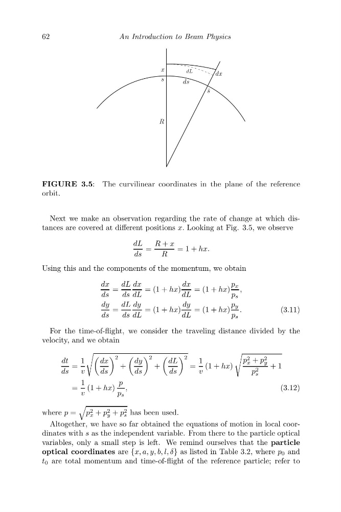
FIGURE 3.5: The curvilinear coordinates in the plane of the reference
orbit.
Next we make an observation regarding the rate of change at which distances are covered at different positions x. Looking at Fig. 3.5, we observe
dL
ds
=
R + x
R
= 1 + hx.
Using this and the components of the momentum, we obtain
dx
ds
=
dL
ds
dx
dL
= (1 + hx)
dx
dL
= (1 + hx)
p x
p s
,
dy
ds
=
dL
ds
dy
dL
= (1 + hx)
dy
dL
= (1 + hx)
p y
p s
.
(3.11)
For the time-of-flight, we consider the traveling distance divided by the
velocity, and we obtain
dt
ds
=
1
v
dx
ds
2
+
dy
ds
2
+
dL
ds
2
=
1
v
(1 + hx)
p 2
x + p 2
y
p 2
s
+ 1
=
1
v
(1 + hx)
p
p s
,
(3.12)
where p =
p 2
x + p 2
y + p 2
s has been used.
Altogether, we have so far obtained the equations of motion in local coordinates with s as the independent variable. From there to the particle optical
variables, only a small step is left. We remind ourselves that the particle
optical coordinates are {x, a, y, b, l, δ} as listed in Table 3.2, where p 0 and
t 0 are total momentum and time-of-flight of the reference particle; refer to
An Introduction to Beam Physics
s
¯
s
ds
R
x
dL
dx
FIGURE 3.5: The curvilinear coordinates in the plane of the reference
orbit.
Next we make an observation regarding the rate of change at which distances are covered at different positions x. Looking at Fig. 3.5, we observe
dL
ds
=
R + x
R
= 1 + hx.
Using this and the components of the momentum, we obtain
dx
ds
=
dL
ds
dx
dL
= (1 + hx)
dx
dL
= (1 + hx)
p x
p s
,
dy
ds
=
dL
ds
dy
dL
= (1 + hx)
dy
dL
= (1 + hx)
p y
p s
.
(3.11)
For the time-of-flight, we consider the traveling distance divided by the
velocity, and we obtain
dt
ds
=
1
v
dx
ds
2
+
dy
ds
2
+
dL
ds
2
=
1
v
(1 + hx)
p 2
x + p 2
y
p 2
s
+ 1
=
1
v
(1 + hx)
p
p s
,
(3.12)
where p =
p 2
x + p 2
y + p 2
s has been used.
Altogether, we have so far obtained the equations of motion in local coordinates with s as the independent variable. From there to the particle optical
variables, only a small step is left. We remind ourselves that the particle
optical coordinates are {x, a, y, b, l, δ} as listed in Table 3.2, where p 0 and
t 0 are total momentum and time-of-flight of the reference particle; refer to