

Fields, Potentials and Equations of Motion
61
where we have used t
= dt/d¯ s, and it is worthwhile to remind ourselves that
the force
F (¯ s) still depends on both x and
p.
As we have progressed from s to ¯
s, the orientation of our locally attached
particle optical coordinate system has changed. It was rotated by the angle
α of eq. (3.9). By using the rotation matrix
ˆ
R(¯ s) =
⎛
⎜
⎝
cos α 0 sinα
0
1
0
− sin α 0 cosα
⎞
⎟
⎠ =
⎛
⎜
⎝
cos
¯
s
s h(¯ s)d¯ s 0 sin
¯
s
s h(¯ s)d¯ s
0
1
0
− sin
¯
s
s h(¯ s)d¯ s 0 cos
¯
s
s h(¯ s)d¯ s
⎞
⎟
⎠ ,
we have the momentum in the new rotated local coordinates
p l (¯ s) = (p x , p y , p s )
as
p l (¯ s) = ˆ
R(¯ s) ·
p(¯ s)
=
⎛
⎜
⎝
cos
¯
s
s
h(¯ s)d¯ s 0 sin
¯
s
s
h(¯ s)d¯ s
0
1
0
− sin
¯
s
s
h(¯ s)d¯ s 0 cos
¯
s
s
h(¯ s)d¯ s
⎞
⎟
⎠ ·
p(s) +
¯
s
s
F (¯ s)t
d¯ s
,
where we have expressed the last line in the integral form. In order to obtain
the rate of change of the momentum
p l , we differentiate with respect to ¯
s.
Noting that
d
d¯ s
sin
¯
s
s
h(¯ s)d¯ s = h(¯ s) cos
¯
s
s
h(¯ s)d¯ s,
d
d¯ s
cos
¯
s
s
h(¯ s)d¯ s = −h(¯ s) sin
¯
s
s
h(¯ s)d¯ s,
evaluate at ¯
s = s and obtain
p l
(s) =
ˆ
R(¯ s)
F (¯ s)t
+ ˆ
R
(¯ s)
p(¯ s) +
¯
s
s
F (¯ s)t
d¯ s
¯
s=s
=
F (s)t
+
⎛
⎝
0
0 h(s)
0
0
0
−h(s) 0
0
⎞
⎠
p(s).
(3.10)
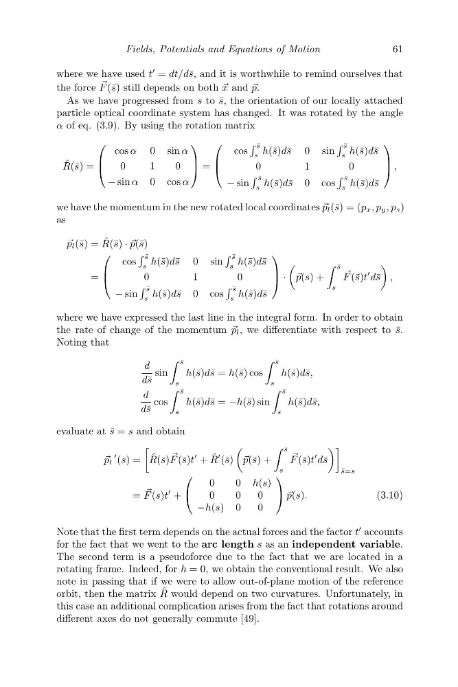
Note that the first term depends on the actual forces and the factor t
accounts
for the fact that we went to the arc length s as an independent variable.
The second term is a pseudoforce due to the fact that we are located in a
rotating frame. Indeed, for h = 0, we obtain the conventional result. We also
note in passing that if we were to allow out-of-plane motion of the reference
orbit, then the matrix ˆ
R would depend on two curvatures. Unfortunately, in
this case an additional complication arises from the fact that rotations around
different axes do not generally commute [49].
61
where we have used t
= dt/d¯ s, and it is worthwhile to remind ourselves that
the force
F (¯ s) still depends on both x and
p.
As we have progressed from s to ¯
s, the orientation of our locally attached
particle optical coordinate system has changed. It was rotated by the angle
α of eq. (3.9). By using the rotation matrix
ˆ
R(¯ s) =
⎛
⎜
⎝
cos α 0 sinα
0
1
0
− sin α 0 cosα
⎞
⎟
⎠ =
⎛
⎜
⎝
cos
¯
s
s h(¯ s)d¯ s 0 sin
¯
s
s h(¯ s)d¯ s
0
1
0
− sin
¯
s
s h(¯ s)d¯ s 0 cos
¯
s
s h(¯ s)d¯ s
⎞
⎟
⎠ ,
we have the momentum in the new rotated local coordinates
p l (¯ s) = (p x , p y , p s )
as
p l (¯ s) = ˆ
R(¯ s) ·
p(¯ s)
=
⎛
⎜
⎝
cos
¯
s
s
h(¯ s)d¯ s 0 sin
¯
s
s
h(¯ s)d¯ s
0
1
0
− sin
¯
s
s
h(¯ s)d¯ s 0 cos
¯
s
s
h(¯ s)d¯ s
⎞
⎟
⎠ ·
p(s) +
¯
s
s
F (¯ s)t
d¯ s
,
where we have expressed the last line in the integral form. In order to obtain
the rate of change of the momentum
p l , we differentiate with respect to ¯
s.
Noting that
d
d¯ s
sin
¯
s
s
h(¯ s)d¯ s = h(¯ s) cos
¯
s
s
h(¯ s)d¯ s,
d
d¯ s
cos
¯
s
s
h(¯ s)d¯ s = −h(¯ s) sin
¯
s
s
h(¯ s)d¯ s,
evaluate at ¯
s = s and obtain
p l
(s) =
ˆ
R(¯ s)
F (¯ s)t
+ ˆ
R
(¯ s)
p(¯ s) +
¯
s
s
F (¯ s)t
d¯ s
¯
s=s
=
F (s)t
+
⎛
⎝
0
0 h(s)
0
0
0
−h(s) 0
0
⎞
⎠
p(s).
(3.10)
Note that the first term depends on the actual forces and the factor t
accounts
for the fact that we went to the arc length s as an independent variable.
The second term is a pseudoforce due to the fact that we are located in a
rotating frame. Indeed, for h = 0, we obtain the conventional result. We also
note in passing that if we were to allow out-of-plane motion of the reference
orbit, then the matrix ˆ
R would depend on two curvatures. Unfortunately, in
this case an additional complication arises from the fact that rotations around
different axes do not generally commute [49].