

56
An Introduction to Beam Physics
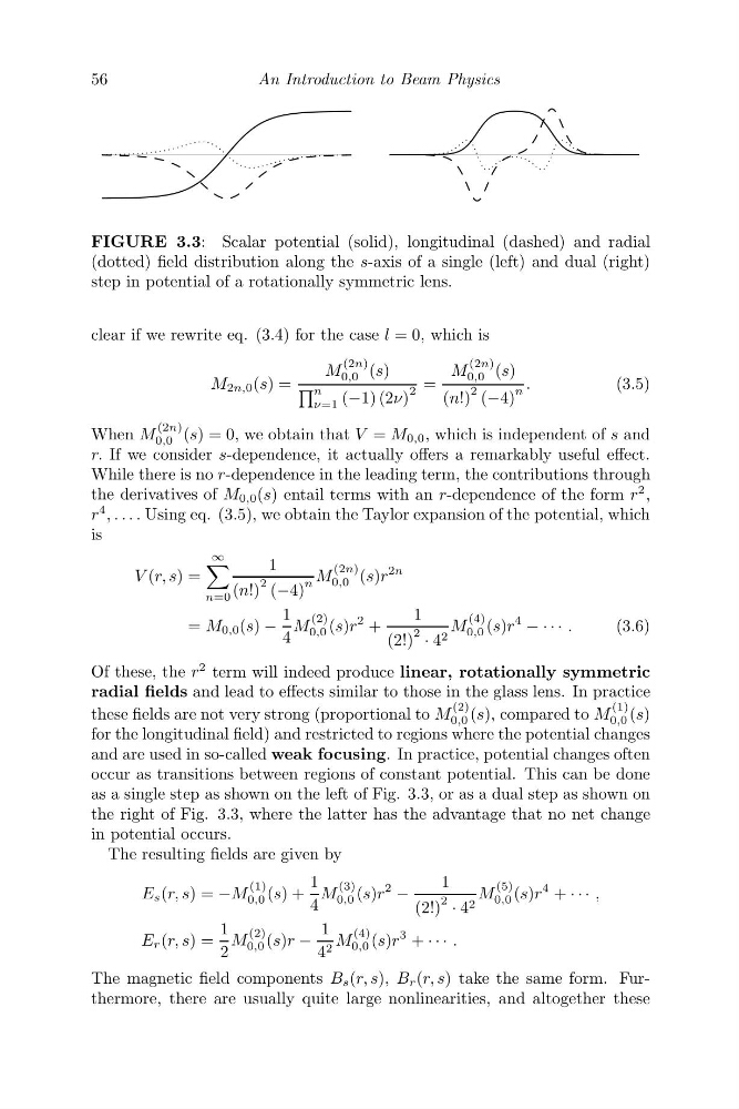
FIGURE 3.3: Scalar potential (solid), longitudinal (dashed) and radial
(dotted) field distribution along the s-axis of a single (left) and dual (right)
step in potential of a rotationally symmetric lens.
clear if we rewrite eq. (3.4) for the case l = 0, which is
M 2n,0 (s) =
M
(2n)
0,0 (s)
n
ν=1 (−1) (2ν)
2 =
M
(2n)
0,0 (s)
(n!)
2 (−4)
n .
(3.5)
When M
(2n)
0,0 (s) = 0, we obtain that V = M 0,0 , which is independent of s and
r. If we consider s-dependence, it actually offers a remarkably useful effect.
While there is no r-dependence in the leading term, the contributions through
the derivatives of M 0,0 (s) entail terms with an r-dependence of the form r
2 ,
r
4 , . . . . Using eq. (3.5), we obtain the Taylor expansion of the potential, which
is
V (r, s) =
∞
n=0
1
(n!)
2 (−4)
n M
(2n)
0,0 (s)r
2n
= M 0,0 (s) −
1
4
M
(2)
0,0 (s)r
2 +
1
(2!)
2 · 4 2
M
(4)
0,0 (s)r
4
− · · · .
(3.6)
Of these, the r
2 term will indeed produce linear, rotationally symmetric
radial fields and lead to effects similar to those in the glass lens. In practice
these fields are not very strong (proportional to M
(2)
0,0 (s), compared to M
(1)
0,0 (s)
for the longitudinal field) and restricted to regions where the potential changes
and are used in so-called weak focusing. In practice, potential changes often
occur as transitions between regions of constant potential. This can be done
as a single step as shown on the left of Fig. 3.3, or as a dual step as shown on
the right of Fig. 3.3, where the latter has the advantage that no net change
in potential occurs.
The resulting fields are given by
E s (r, s) = −M
(1)
0,0 (s) +
1
4
M
(3)
0,0 (s)r
2
−
1
(2!)
2 · 4 2
M
(5)
0,0 (s)r
4 + · · · ,
E r (r, s) =
1
2
M
(2)
0,0 (s)r −
1
4 2 M
(4)
0,0 (s)r
3 + · · · .
The magnetic field components B s (r, s), B r (r, s) take the same form. Furthermore, there are usually quite large nonlinearities, and altogether these
An Introduction to Beam Physics
FIGURE 3.3: Scalar potential (solid), longitudinal (dashed) and radial
(dotted) field distribution along the s-axis of a single (left) and dual (right)
step in potential of a rotationally symmetric lens.
clear if we rewrite eq. (3.4) for the case l = 0, which is
M 2n,0 (s) =
M
(2n)
0,0 (s)
n
ν=1 (−1) (2ν)
2 =
M
(2n)
0,0 (s)
(n!)
2 (−4)
n .
(3.5)
When M
(2n)
0,0 (s) = 0, we obtain that V = M 0,0 , which is independent of s and
r. If we consider s-dependence, it actually offers a remarkably useful effect.
While there is no r-dependence in the leading term, the contributions through
the derivatives of M 0,0 (s) entail terms with an r-dependence of the form r
2 ,
r
4 , . . . . Using eq. (3.5), we obtain the Taylor expansion of the potential, which
is
V (r, s) =
∞
n=0
1
(n!)
2 (−4)
n M
(2n)
0,0 (s)r
2n
= M 0,0 (s) −
1
4
M
(2)
0,0 (s)r
2 +
1
(2!)
2 · 4 2
M
(4)
0,0 (s)r
4
− · · · .
(3.6)
Of these, the r
2 term will indeed produce linear, rotationally symmetric
radial fields and lead to effects similar to those in the glass lens. In practice
these fields are not very strong (proportional to M
(2)
0,0 (s), compared to M
(1)
0,0 (s)
for the longitudinal field) and restricted to regions where the potential changes
and are used in so-called weak focusing. In practice, potential changes often
occur as transitions between regions of constant potential. This can be done
as a single step as shown on the left of Fig. 3.3, or as a dual step as shown on
the right of Fig. 3.3, where the latter has the advantage that no net change
in potential occurs.
The resulting fields are given by
E s (r, s) = −M
(1)
0,0 (s) +
1
4
M
(3)
0,0 (s)r
2
−
1
(2!)
2 · 4 2
M
(5)
0,0 (s)r
4 + · · · ,
E r (r, s) =
1
2
M
(2)
0,0 (s)r −
1
4 2 M
(4)
0,0 (s)r
3 + · · · .
The magnetic field components B s (r, s), B r (r, s) take the same form. Furthermore, there are usually quite large nonlinearities, and altogether these