

Resonances in Repetitive Systems
281
11.4 Third–Integer Resonance
In this section we deal with the third–integer resonance, which is generated
by the sextupoles introduced into the ring to compensate for chromaticity.
Similar to the previous section, we will start with a particle with an arbitrary
position and angle and demonstrate the resonant behavior when the tune
is close to the resonance. Again, let us first consider the case that a thin
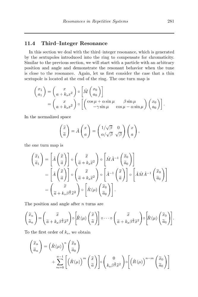
sextupole is located at the end of the ring. The one turn map is
x 1
a 1
=
x
a + k s x
2
◦
ˆ
M
x 0
a 0
=
x
a + k s x
2
◦
cos μ + α sin μ
βsin μ
−γ sin μ
cos μ − α sin μ
x 0
a 0
.
In the normalized space
x
a
= ˆ
A
x
a
=
1/
√
β 0
α/
√
β
√
β
x
a
,
the one turn map is
x 1
a 1
=
ˆ
A
x
a
◦
x
a + k s
x
2
◦
ˆ
M ˆ
A
−1
x 0
a 0
=
ˆ
A
x
a
◦
x
a + k s
x
2
◦
ˆ
A
−1
x
a
◦
ˆ
A ˆ
M ˆ
A
−1
x 0
a 0
=
x
a + k s β
3
2
x
2
◦
ˆ
R (μ)
x 0
a 0
.
The position and angle after n turns are
x n
a n
=
x
a + k s β
3
2
x
2
◦
ˆ
R (μ)
x
a
◦ · · · ◦
x
a + k s β
3
2
x
2
◦
ˆ
R (μ)
x 0
a 0
.
To the first order of k s , we obtain
x n
a n
=
ˆ
R (μ)
n
x 0
a 0
+
n−1
m=0
ˆ
R (μ)
m
x
a
◦
0
k s β
3
2
x
2
◦
ˆ
R (μ)
n−m
x 0
a 0
281
11.4 Third–Integer Resonance
In this section we deal with the third–integer resonance, which is generated
by the sextupoles introduced into the ring to compensate for chromaticity.
Similar to the previous section, we will start with a particle with an arbitrary
position and angle and demonstrate the resonant behavior when the tune
is close to the resonance. Again, let us first consider the case that a thin
sextupole is located at the end of the ring. The one turn map is
x 1
a 1
=
x
a + k s x
2
◦
ˆ
M
x 0
a 0
=
x
a + k s x
2
◦
cos μ + α sin μ
βsin μ
−γ sin μ
cos μ − α sin μ
x 0
a 0
.
In the normalized space
x
a
= ˆ
A
x
a
=
1/
√
β 0
α/
√
β
√
β
x
a
,
the one turn map is
x 1
a 1
=
ˆ
A
x
a
◦
x
a + k s
x
2
◦
ˆ
M ˆ
A
−1
x 0
a 0
=
ˆ
A
x
a
◦
x
a + k s
x
2
◦
ˆ
A
−1
x
a
◦
ˆ
A ˆ
M ˆ
A
−1
x 0
a 0
=
x
a + k s β
3
2
x
2
◦
ˆ
R (μ)
x 0
a 0
.
The position and angle after n turns are
x n
a n
=
x
a + k s β
3
2
x
2
◦
ˆ
R (μ)
x
a
◦ · · · ◦
x
a + k s β
3
2
x
2
◦
ˆ
R (μ)
x 0
a 0
.
To the first order of k s , we obtain
x n
a n
=
ˆ
R (μ)
n
x 0
a 0
+
n−1
m=0
ˆ
R (μ)
m
x
a
◦
0
k s β
3
2
x
2
◦
ˆ
R (μ)
n−m
x 0
a 0