

Synchrotron Motion
249
V, ΔE k
V, ΔE k
φ
φ
-φ s
φ s
π
2π
3π
0
π
2π
3π
0
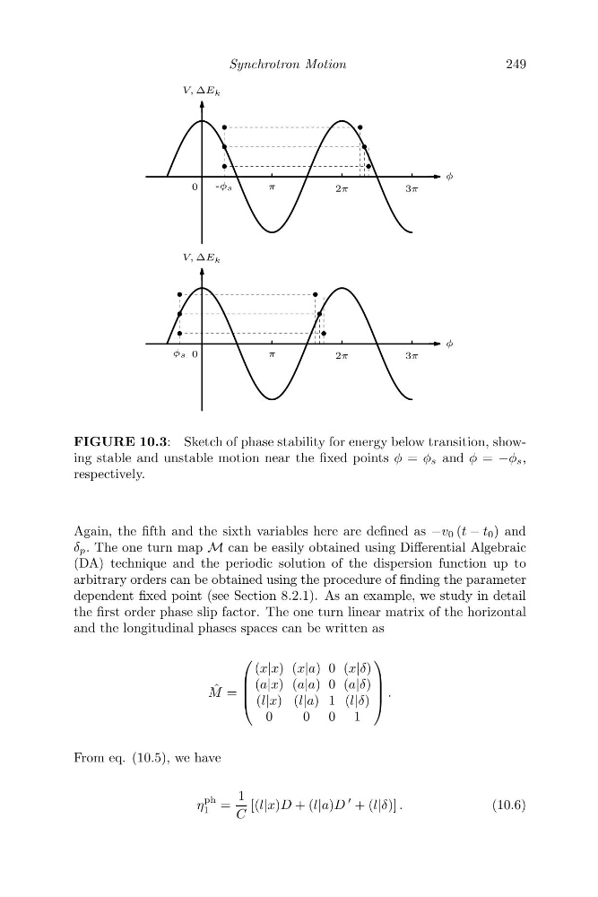
FIGURE 10.3: Sketch of phase stability for energy below transition, showing stable and unstable motion near the fixed points φ = φ s and φ = −φ s ,
respectively.
Again, the fifth and the sixth variables here are defined as −v 0 (t − t 0 ) and
δ p . The one turn map M can be easily obtained using Differential Algebraic
(DA) technique and the periodic solution of the dispersion function up to
arbitrary orders can be obtained using the procedure of finding the parameter
dependent fixed point (see Section 8.2.1). As an example, we study in detail
the first order phase slip factor. The one turn linear matrix of the horizontal
and the longitudinal phases spaces can be written as
ˆ
M =
⎛
⎜
⎜
⎝
(x|x) (x|a) 0 (x|δ)
(a|x) (a|a) 0 (a|δ)
(l|x) (l|a) 1 (l|δ)
0
0 0 1
⎞
⎟
⎟
⎠ .
From eq. (10.5), we have
η
ph
1 =
1
C
[(l|x)D + (l|a)D
+ (l|δ)] .
(10.6)
249
V, ΔE k
V, ΔE k
φ
φ
-φ s
φ s
π
2π
3π
0
π
2π
3π
0
FIGURE 10.3: Sketch of phase stability for energy below transition, showing stable and unstable motion near the fixed points φ = φ s and φ = −φ s ,
respectively.
Again, the fifth and the sixth variables here are defined as −v 0 (t − t 0 ) and
δ p . The one turn map M can be easily obtained using Differential Algebraic
(DA) technique and the periodic solution of the dispersion function up to
arbitrary orders can be obtained using the procedure of finding the parameter
dependent fixed point (see Section 8.2.1). As an example, we study in detail
the first order phase slip factor. The one turn linear matrix of the horizontal
and the longitudinal phases spaces can be written as
ˆ
M =
⎛
⎜
⎜
⎝
(x|x) (x|a) 0 (x|δ)
(a|x) (a|a) 0 (a|δ)
(l|x) (l|a) 1 (l|δ)
0
0 0 1
⎞
⎟
⎟
⎠ .
From eq. (10.5), we have
η
ph
1 =
1
C
[(l|x)D + (l|a)D
+ (l|δ)] .
(10.6)