

180
An Introduction to Beam Physics
The linear optics consists of two identical quadrupole doublets with equal
spacing between the quadrupoles and equal strength of all quadrupoles. The
two outer octupoles correct the terms (x|a
3 ) and (y|b
3 ), and the middle one
corrects (x|ab
2 ) and (y|a
2 b). Due to the large difference in transverse position
of the horizontal and vertical rays in the outer octupoles, the two knobs are
mostly orthogonal. A resolution of 0.78 ˚
A has been achieved using such a
corrector.
While the introduction of the C S corrector into an electron microscope
corrects the third order spherical aberration, it also generates much larger
fifth order spherical aberrations (C 5 ) through the combination of the
objective lens and the octupoles and that among the octupoles, which becomes
the limiting factor as the resolution reaches toward 0.5 ˚
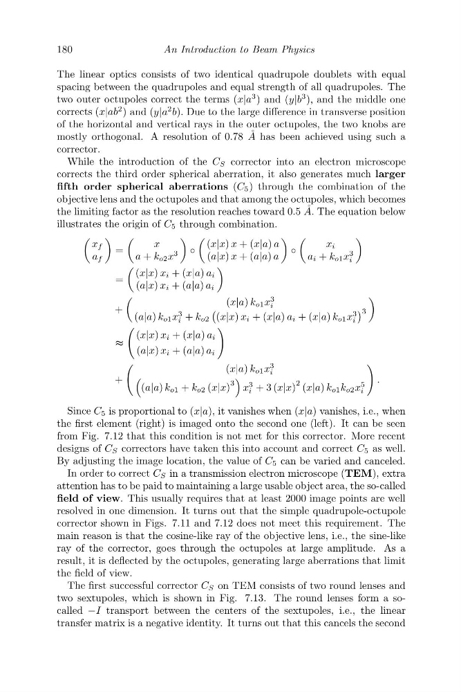
A. The equation below
illustrates the origin of C 5 through combination.
x f
a f
=
x
a + k o2 x
3
◦
(x|x) x + (x|a) a
(a|x) x + (a|a) a
◦
x i
a i + k o1 x
3
i
=
(x|x) x i + (x|a) a i
(a|x) x i + (a|a) a i
+
(x|a) k o1 x
3
i
(a|a) k o1 x
3
i + k o2
(x|x) x i + (x|a) a i + (x|a) k o1 x
3
i
3
≈
(x|x) x i + (x|a) a i
(a|x) x i + (a|a) a i
+
(x|a) k o1 x
3
i
(a|a) k o1 + k o2 (x|x)
3
x
3
i + 3 (x|x)
2 (x|a) k o1 k o2 x
5
i
.
Since C 5 is proportional to (x|a), it vanishes when (x|a) vanishes, i.e., when
the first element (right) is imaged onto the second one (left). It can be seen
from Fig. 7.12 that this condition is not met for this corrector. More recent
designs of C S correctors have taken this into account and correct C 5 as well.
By adjusting the image location, the value of C 5 can be varied and canceled.
In order to correct C S in a transmission electron microscope (TEM), extra
attention has to be paid to maintaining a large usable object area, the so-called
field of view. This usually requires that at least 2000 image points are well
resolved in one dimension. It turns out that the simple quadrupole-octupole
corrector shown in Figs. 7.11 and 7.12 does not meet this requirement. The
main reason is that the cosine-like ray of the objective lens, i.e., the sine-like
ray of the corrector, goes through the octupoles at large amplitude. As a
result, it is deflected by the octupoles, generating large aberrations that limit
the field of view.
The first successful corrector C S on TEM consists of two round lenses and
two sextupoles, which is shown in Fig. 7.13. The round lenses form a socalled −I transport between the centers of the sextupoles, i.e., the linear
transfer matrix is a negative identity. It turns out that this cancels the second
An Introduction to Beam Physics
The linear optics consists of two identical quadrupole doublets with equal
spacing between the quadrupoles and equal strength of all quadrupoles. The
two outer octupoles correct the terms (x|a
3 ) and (y|b
3 ), and the middle one
corrects (x|ab
2 ) and (y|a
2 b). Due to the large difference in transverse position
of the horizontal and vertical rays in the outer octupoles, the two knobs are
mostly orthogonal. A resolution of 0.78 ˚
A has been achieved using such a
corrector.
While the introduction of the C S corrector into an electron microscope
corrects the third order spherical aberration, it also generates much larger
fifth order spherical aberrations (C 5 ) through the combination of the
objective lens and the octupoles and that among the octupoles, which becomes
the limiting factor as the resolution reaches toward 0.5 ˚
A. The equation below
illustrates the origin of C 5 through combination.
x f
a f
=
x
a + k o2 x
3
◦
(x|x) x + (x|a) a
(a|x) x + (a|a) a
◦
x i
a i + k o1 x
3
i
=
(x|x) x i + (x|a) a i
(a|x) x i + (a|a) a i
+
(x|a) k o1 x
3
i
(a|a) k o1 x
3
i + k o2
(x|x) x i + (x|a) a i + (x|a) k o1 x
3
i
3
≈
(x|x) x i + (x|a) a i
(a|x) x i + (a|a) a i
+
(x|a) k o1 x
3
i
(a|a) k o1 + k o2 (x|x)
3
x
3
i + 3 (x|x)
2 (x|a) k o1 k o2 x
5
i
.
Since C 5 is proportional to (x|a), it vanishes when (x|a) vanishes, i.e., when
the first element (right) is imaged onto the second one (left). It can be seen
from Fig. 7.12 that this condition is not met for this corrector. More recent
designs of C S correctors have taken this into account and correct C 5 as well.
By adjusting the image location, the value of C 5 can be varied and canceled.
In order to correct C S in a transmission electron microscope (TEM), extra
attention has to be paid to maintaining a large usable object area, the so-called
field of view. This usually requires that at least 2000 image points are well
resolved in one dimension. It turns out that the simple quadrupole-octupole
corrector shown in Figs. 7.11 and 7.12 does not meet this requirement. The
main reason is that the cosine-like ray of the objective lens, i.e., the sine-like
ray of the corrector, goes through the octupoles at large amplitude. As a
result, it is deflected by the octupoles, generating large aberrations that limit
the field of view.
The first successful corrector C S on TEM consists of two round lenses and
two sextupoles, which is shown in Fig. 7.13. The round lenses form a socalled −I transport between the centers of the sextupoles, i.e., the linear
transfer matrix is a negative identity. It turns out that this cancels the second