

174
An Introduction to Beam Physics
placing magnetic multipoles of the same order into the system. They are either separate adjustable multipoles or combined fixed elements to dipoles or
quadrupoles.
7.3.2 Energy Loss On–Line Isotope Separators
As part of the growing developments in the study of radioactive beams, on–
line isotope separation is more and more widely performed. As in other
mass spectrometers described above, different isotopes have to be laterally
separated. Yet they can no longer be bent by electrostatic sectors anymore
due to their high energy. Among the different methods, the energy loss method
is a very interesting one. First, particles of the right rigidity are selected by
a slit at the dispersive focal point. Second, the selected particles are sent
through an energy degrader which creates new momentum spread according
to the mass of the particles. And finally, a second slit picks up the desired
nuclei. The best spatial separation can be achieved when the whole beamline
is achromatic and the degrader preserves the achromaticity. This is due to
the fact that nuclei of the same mass but different momentum are focused at
the same spot. Hence it is important to study the transfer map of an energy
degrader and the achromatic conditions.
In most of the cases, the degrader is thin enough for us to neglect the
straggling effect from multiple scattering. So a degrader is the combination
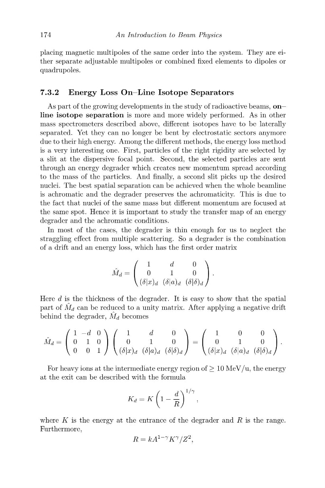
of a drift and an energy loss, which has the first order matrix
ˆ
M d =
⎛
⎝
1
d
0
0
1
0
(δ|x) d (δ|a) d (δ|δ) d
⎞
⎠ .
Here d is the thickness of the degrader. It is easy to show that the spatial
part of ˆ
M d can be reduced to a unity matrix. After applying a negative drift
behind the degrader, ˆ
M d becomes
ˆ
M d =
⎛
⎝
1 −d 0
0 1 0
0 0 1
⎞
⎠
⎛
⎝
1
d
0
0
1
0
(δ|x) d (δ|a) d (δ|δ) d
⎞
⎠ =
⎛
⎝
1
0
0
0
1
0
(δ|x) d (δ|a) d (δ|δ) d
⎞
⎠ .
For heavy ions at the intermediate energy region of ≥ 10 MeV/u, the energy
at the exit can be described with the formula
K d = K
1 −
d
R
1/γ
,
where K is the energy at the entrance of the degrader and R is the range.
Furthermore,
R = kA
1−γ K
γ /Z
2 ,
An Introduction to Beam Physics
placing magnetic multipoles of the same order into the system. They are either separate adjustable multipoles or combined fixed elements to dipoles or
quadrupoles.
7.3.2 Energy Loss On–Line Isotope Separators
As part of the growing developments in the study of radioactive beams, on–
line isotope separation is more and more widely performed. As in other
mass spectrometers described above, different isotopes have to be laterally
separated. Yet they can no longer be bent by electrostatic sectors anymore
due to their high energy. Among the different methods, the energy loss method
is a very interesting one. First, particles of the right rigidity are selected by
a slit at the dispersive focal point. Second, the selected particles are sent
through an energy degrader which creates new momentum spread according
to the mass of the particles. And finally, a second slit picks up the desired
nuclei. The best spatial separation can be achieved when the whole beamline
is achromatic and the degrader preserves the achromaticity. This is due to
the fact that nuclei of the same mass but different momentum are focused at
the same spot. Hence it is important to study the transfer map of an energy
degrader and the achromatic conditions.
In most of the cases, the degrader is thin enough for us to neglect the
straggling effect from multiple scattering. So a degrader is the combination
of a drift and an energy loss, which has the first order matrix
ˆ
M d =
⎛
⎝
1
d
0
0
1
0
(δ|x) d (δ|a) d (δ|δ) d
⎞
⎠ .
Here d is the thickness of the degrader. It is easy to show that the spatial
part of ˆ
M d can be reduced to a unity matrix. After applying a negative drift
behind the degrader, ˆ
M d becomes
ˆ
M d =
⎛
⎝
1 −d 0
0 1 0
0 0 1
⎞
⎠
⎛
⎝
1
d
0
0
1
0
(δ|x) d (δ|a) d (δ|δ) d
⎞
⎠ =
⎛
⎝
1
0
0
0
1
0
(δ|x) d (δ|a) d (δ|δ) d
⎞
⎠ .
For heavy ions at the intermediate energy region of ≥ 10 MeV/u, the energy
at the exit can be described with the formula
K d = K
1 −
d
R
1/γ
,
where K is the energy at the entrance of the degrader and R is the range.
Furthermore,
R = kA
1−γ K
γ /Z
2 ,