

Imaging Devices
167
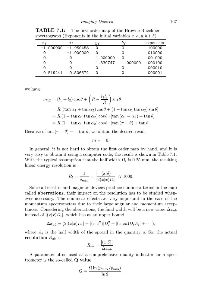
TABLE 7.1: The first order map of the Browne-Buechner
spectrograph (Exponents in the initial variables x, a, y, b, l, δ)
x f
a f
y f
b f
exponents
-1.000000 -1.950458
0
0
100000
0
-1.000000
0
0
010000
0
0
1.000000
0
001000
0
0
1.830747
1.000000
000100
0
0
0
0
000010
0.519441
0.506574
0
0
000001
we have
m 12 = (l 1 + l 2 ) cos θ +
R −
l 1 l 2
R
sin θ
= R [(tan α 1 + tan α 2 ) cos θ + (1 − tan α 1 tan α 2 ) sin θ]
= R (1 − tan α 1 tan α 2 ) cos θ · [tan (α 1 + α 2 ) + tan θ]
= R (1 − tan α 1 tan α 2 ) cos θ · [tan (π − θ) + tan θ] .
Because of tan (π − θ) = − tan θ, we obtain the desired result
m 12 = 0.
In general, it is not hard to obtain the first order map by hand, and it is
very easy to obtain it using a computer code; the result is shown in Table 7.1.
With the typical assumption that the half width D i is 0.25 mm, the resulting
linear energy resolution is
R l =
1
δ min
=
(x|δ)
2(x|x)D i
≈ 1000.
Since all electric and magnetic devices produce nonlinear terms in the map
called aberrations, their impact on the resolution has to be studied whenever necessary. The nonlinear effects are very important in the case of the
momentum spectrometers due to their large angular and momentum acceptances. Considering the aberrations, the final width will be a new value Δx ab
instead of |(x|x)D i |, which has as an upper bound
Δx ab = (2|(x|x)D i | + |(x|x
2 )|D
2
i + |(x|xa)D i A i | + · · · ),
where A i is the half width of the spread in the quantity a. So, the actual
resolution R ab is
R ab =
|(x|δ)|
Δx ab
.
A parameter often used as a comprehensive quality indicator for a spectrometer is the so-called Q value
Q =
Ω ln (p max /p min )
ln 2
,
167
TABLE 7.1: The first order map of the Browne-Buechner
spectrograph (Exponents in the initial variables x, a, y, b, l, δ)
x f
a f
y f
b f
exponents
-1.000000 -1.950458
0
0
100000
0
-1.000000
0
0
010000
0
0
1.000000
0
001000
0
0
1.830747
1.000000
000100
0
0
0
0
000010
0.519441
0.506574
0
0
000001
we have
m 12 = (l 1 + l 2 ) cos θ +
R −
l 1 l 2
R
sin θ
= R [(tan α 1 + tan α 2 ) cos θ + (1 − tan α 1 tan α 2 ) sin θ]
= R (1 − tan α 1 tan α 2 ) cos θ · [tan (α 1 + α 2 ) + tan θ]
= R (1 − tan α 1 tan α 2 ) cos θ · [tan (π − θ) + tan θ] .
Because of tan (π − θ) = − tan θ, we obtain the desired result
m 12 = 0.
In general, it is not hard to obtain the first order map by hand, and it is
very easy to obtain it using a computer code; the result is shown in Table 7.1.
With the typical assumption that the half width D i is 0.25 mm, the resulting
linear energy resolution is
R l =
1
δ min
=
(x|δ)
2(x|x)D i
≈ 1000.
Since all electric and magnetic devices produce nonlinear terms in the map
called aberrations, their impact on the resolution has to be studied whenever necessary. The nonlinear effects are very important in the case of the
momentum spectrometers due to their large angular and momentum acceptances. Considering the aberrations, the final width will be a new value Δx ab
instead of |(x|x)D i |, which has as an upper bound
Δx ab = (2|(x|x)D i | + |(x|x
2 )|D
2
i + |(x|xa)D i A i | + · · · ),
where A i is the half width of the spread in the quantity a. So, the actual
resolution R ab is
R ab =
|(x|δ)|
Δx ab
.
A parameter often used as a comprehensive quality indicator for a spectrometer is the so-called Q value
Q =
Ω ln (p max /p min )
ln 2
,