

166
An Introduction to Beam Physics
α 1
α 2
θ
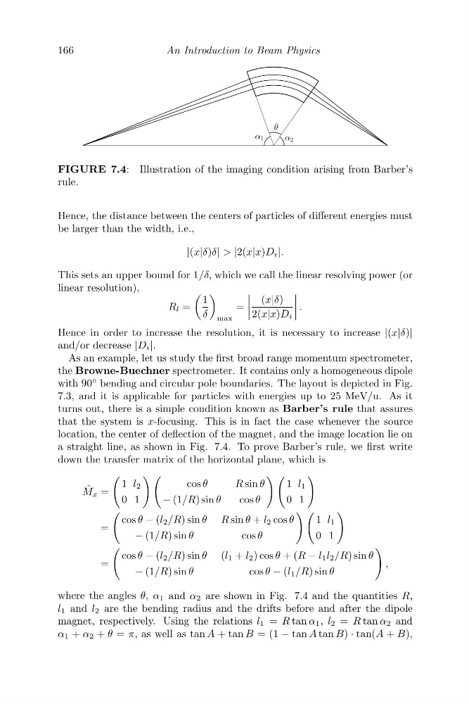
FIGURE 7.4: Illustration of the imaging condition arising from Barber’s
rule.
Hence, the distance between the centers of particles of different energies must
be larger than the width, i.e.,
|(x|δ)δ| > |2(x|x)D i |.
This sets an upper bound for 1/δ, which we call the linear resolving power (or
linear resolution),
R l =
1
δ
max
=
(x|δ)
2(x|x)D i
.
Hence in order to increase the resolution, it is necessary to increase |(x|δ)|
and/or decrease |D i |.
As an example, let us study the first broad range momentum spectrometer,
the Browne-Buechner spectrometer. It contains only a homogeneous dipole
with 90
◦ bending and circular pole boundaries. The layout is depicted in Fig.
7.3, and it is applicable for particles with energies up to 25 MeV/u. As it
turns out, there is a simple condition known as Barber’s rule that assures
that the system is x-focusing. This is in fact the case whenever the source
location, the center of deflection of the magnet, and the image location lie on
a straight line, as shown in Fig. 7.4. To prove Barber’s rule, we first write
down the transfer matrix of the horizontal plane, which is
ˆ
M x =
1 l 2
0 1
cos θ
Rsin θ
− (1/R) sin θ
cos θ
1 l 1
0 1
=
cos θ − (l 2 /R) sin θ Rsin θ + l 2 cos θ
− (1/R) sin θ
cos θ
1 l 1
0 1
=
cos θ − (l 2 /R) sin θ (l 1 + l 2 ) cos θ + (R − l 1 l 2 /R) sin θ
− (1/R) sin θ
cos θ − (l 1 /R) sin θ
,
where the angles θ, α 1 and α 2 are shown in Fig. 7.4 and the quantities R,
l 1 and l 2 are the bending radius and the drifts before and after the dipole
magnet, respectively. Using the relations l 1 = R tan α 1 , l 2 = R tan α 2 and
α 1 + α 2 + θ = π, as well as tan A + tan B = (1 − tan A tan B) · tan(A + B),
An Introduction to Beam Physics
α 1
α 2
θ
FIGURE 7.4: Illustration of the imaging condition arising from Barber’s
rule.
Hence, the distance between the centers of particles of different energies must
be larger than the width, i.e.,
|(x|δ)δ| > |2(x|x)D i |.
This sets an upper bound for 1/δ, which we call the linear resolving power (or
linear resolution),
R l =
1
δ
max
=
(x|δ)
2(x|x)D i
.
Hence in order to increase the resolution, it is necessary to increase |(x|δ)|
and/or decrease |D i |.
As an example, let us study the first broad range momentum spectrometer,
the Browne-Buechner spectrometer. It contains only a homogeneous dipole
with 90
◦ bending and circular pole boundaries. The layout is depicted in Fig.
7.3, and it is applicable for particles with energies up to 25 MeV/u. As it
turns out, there is a simple condition known as Barber’s rule that assures
that the system is x-focusing. This is in fact the case whenever the source
location, the center of deflection of the magnet, and the image location lie on
a straight line, as shown in Fig. 7.4. To prove Barber’s rule, we first write
down the transfer matrix of the horizontal plane, which is
ˆ
M x =
1 l 2
0 1
cos θ
Rsin θ
− (1/R) sin θ
cos θ
1 l 1
0 1
=
cos θ − (l 2 /R) sin θ Rsin θ + l 2 cos θ
− (1/R) sin θ
cos θ
1 l 1
0 1
=
cos θ − (l 2 /R) sin θ (l 1 + l 2 ) cos θ + (R − l 1 l 2 /R) sin θ
− (1/R) sin θ
cos θ − (l 1 /R) sin θ
,
where the angles θ, α 1 and α 2 are shown in Fig. 7.4 and the quantities R,
l 1 and l 2 are the bending radius and the drifts before and after the dipole
magnet, respectively. Using the relations l 1 = R tan α 1 , l 2 = R tan α 2 and
α 1 + α 2 + θ = π, as well as tan A + tan B = (1 − tan A tan B) · tan(A + B),