

136
An Introduction to Beam Physics
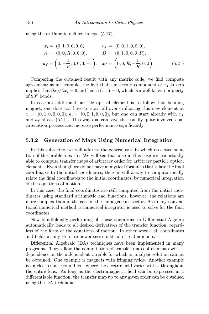
using the arithmetic defined in eqs. (5.17),
x i = (0, 1, 0, 0, 0, 0),
a i = (0, 0, 1, 0, 0, 0),
A = (0, 0, R, 0, 0, 0),
B = (0, 1, 0, 0, 0, R),
a f =
0, −
1
R
, 0, 0, 0, −1
, x f =
0, 0, R, −
1
R
, 0, 0
.
(5.21)
Comparing the obtained result with any matrix code, we find complete
agreement; as an example, the fact that the second component of x f is zero
implies that ∂x f /∂x i = 0 and hence (x|x) = 0, which is a well known property
of 90
◦ bends.
In case an additional particle optical element is to follow this bending
magnet, one does not have to start all over evaluating this new element at
x i = (0, 1, 0, 0, 0, 0), a i = (0, 0, 1, 0, 0, 0), but one can start already with x f
and a f of eq. (5.21). This way one can save the usually quite involved concatenation process and increase performance significantly.
5.3.2 Generation of Maps Using Numerical Integration
In this subsection we will address the general case in which no closed solution of the problem exists. We will see that also in this case we are actually
able to compute transfer maps of arbitrary order for arbitrary particle optical
elements. Even though we do not have analytical formulas that relate the final
coordinates to the initial coordinates, there is still a way to computationally
relate the final coordinates to the initial coordinates, by numerical integration
of the equations of motion.
In this case, the final coordinates are still computed from the initial coordinates using standard arithmetic and functions; however, the relations are
more complex than in the case of the homogeneous sector. As in any conventional numerical method, a numerical integrator is used to solve for the final
coordinates.
Now blindfoldedly performing all these operations in Differential Algebra
automatically leads to all desired derivatives of the transfer function, regardless of the form of the equations of motion. In other words, all coordinates
and fields at any step are power series instead of real numbers.
Differential Algebraic (DA) techniques have been implemented in many
programs. They allow the computation of transfer maps of elements with a
dependence on the independent variable for which an analytic solution cannot
be obtained. One example is magnets with fringing fields. Another example
is an electrostatic round lens where the electric field varies with s throughout
the entire lens. As long as the electromagnetic field can be expressed in a
differentiable function, the transfer map up to any given order can be obtained
using the DA technique.
An Introduction to Beam Physics
using the arithmetic defined in eqs. (5.17),
x i = (0, 1, 0, 0, 0, 0),
a i = (0, 0, 1, 0, 0, 0),
A = (0, 0, R, 0, 0, 0),
B = (0, 1, 0, 0, 0, R),
a f =
0, −
1
R
, 0, 0, 0, −1
, x f =
0, 0, R, −
1
R
, 0, 0
.
(5.21)
Comparing the obtained result with any matrix code, we find complete
agreement; as an example, the fact that the second component of x f is zero
implies that ∂x f /∂x i = 0 and hence (x|x) = 0, which is a well known property
of 90
◦ bends.
In case an additional particle optical element is to follow this bending
magnet, one does not have to start all over evaluating this new element at
x i = (0, 1, 0, 0, 0, 0), a i = (0, 0, 1, 0, 0, 0), but one can start already with x f
and a f of eq. (5.21). This way one can save the usually quite involved concatenation process and increase performance significantly.
5.3.2 Generation of Maps Using Numerical Integration
In this subsection we will address the general case in which no closed solution of the problem exists. We will see that also in this case we are actually
able to compute transfer maps of arbitrary order for arbitrary particle optical
elements. Even though we do not have analytical formulas that relate the final
coordinates to the initial coordinates, there is still a way to computationally
relate the final coordinates to the initial coordinates, by numerical integration
of the equations of motion.
In this case, the final coordinates are still computed from the initial coordinates using standard arithmetic and functions; however, the relations are
more complex than in the case of the homogeneous sector. As in any conventional numerical method, a numerical integrator is used to solve for the final
coordinates.
Now blindfoldedly performing all these operations in Differential Algebra
automatically leads to all desired derivatives of the transfer function, regardless of the form of the equations of motion. In other words, all coordinates
and fields at any step are power series instead of real numbers.
Differential Algebraic (DA) techniques have been implemented in many
programs. They allow the computation of transfer maps of elements with a
dependence on the independent variable for which an analytic solution cannot
be obtained. One example is magnets with fringing fields. Another example
is an electrostatic round lens where the electric field varies with s throughout
the entire lens. As long as the electromagnetic field can be expressed in a
differentiable function, the transfer map up to any given order can be obtained
using the DA technique.