

Computation and Properties of Maps
135
R
R
R
R
x i
x f
α i
α f
(A, B)
(0, 0)
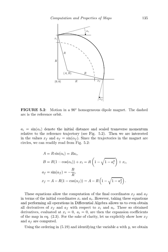
FIGURE 5.2: Motion in a 90
◦ homogeneous dipole magnet. The dashed
arc is the reference orbit.
a i = sin(α i ) denote the initial distance and scaled transverse momentum
relative to the reference trajectory (see Fig. 5.2). Then we are interested
in the values x f and a f = sin(α f ). Since the trajectories in the magnet are
circles, we can readily read from Fig. 5.2:
A = R sin(α i ) = Ra i ,
B = R(1 − cos(α i )) + x i = R
1 −
1 − a 2
i
+ x i ,
a f = sin(α f ) = −
B
R
,
x f = A − R(1 − cos(α f )) = A − R
1 −
1 − a 2
f
.
These equations allow the computation of the final coordinates x f and a f
in terms of the initial coordinates x i and a i . However, taking these equations
and performing all operations in Differential Algebra allows us to even obtain
all derivatives of x f and a f with respect to x i and a i . These so obtained
derivatives, evaluated at x i = 0, a i = 0, are then the expansion coefficients
of the map in eq. (2.3). For the sake of clarity, let us explicitly show how x f
and a f are computed.
Using the ordering in (5.19) and identifying the variable a with y, we obtain
135
R
R
R
R
x i
x f
α i
α f
(A, B)
(0, 0)
FIGURE 5.2: Motion in a 90
◦ homogeneous dipole magnet. The dashed
arc is the reference orbit.
a i = sin(α i ) denote the initial distance and scaled transverse momentum
relative to the reference trajectory (see Fig. 5.2). Then we are interested
in the values x f and a f = sin(α f ). Since the trajectories in the magnet are
circles, we can readily read from Fig. 5.2:
A = R sin(α i ) = Ra i ,
B = R(1 − cos(α i )) + x i = R
1 −
1 − a 2
i
+ x i ,
a f = sin(α f ) = −
B
R
,
x f = A − R(1 − cos(α f )) = A − R
1 −
1 − a 2
f
.
These equations allow the computation of the final coordinates x f and a f
in terms of the initial coordinates x i and a i . However, taking these equations
and performing all operations in Differential Algebra allows us to even obtain
all derivatives of x f and a f with respect to x i and a i . These so obtained
derivatives, evaluated at x i = 0, a i = 0, are then the expansion coefficients
of the map in eq. (2.3). For the sake of clarity, let us explicitly show how x f
and a f are computed.
Using the ordering in (5.19) and identifying the variable a with y, we obtain