

134
An Introduction to Beam Physics
which also holds for DA numbers and leads to simplifications by virtue of eq.
(5.20).
As the last example, we will derive a formula for the root function. Even
though there is a direct method to compute roots by solving a set of linear
equations for the coefficients of the root, we present here a technique based on
power series following an approach similar to the exponential and logarithm.
The root has the following power series expansion:
√
1 + x =
∞
i=0
(−1)
i 1 · 3 · · · (2i − 3)
2 · 4 · · · (2i)
· x
i .
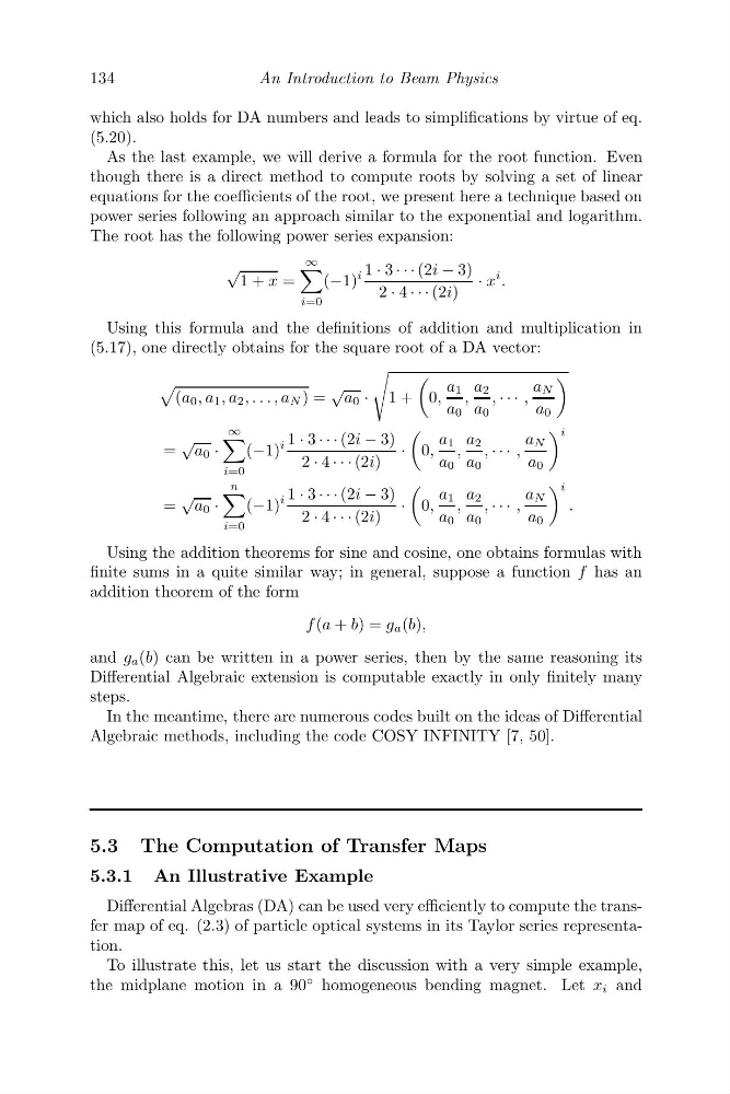
Using this formula and the definitions of addition and multiplication in
(5.17), one directly obtains for the square root of a DA vector:
(a 0 , a 1 , a 2 , . . . , a N ) =
√
a 0 ·
1 +
0,
a 1
a 0
,
a 2
a 0
, · · · ,
a N
a 0
=
√
a 0 ·
∞
i=0
(−1)
i 1 · 3 · · · (2i − 3)
2 · 4 · · · (2i)
·
0,
a 1
a 0
,
a 2
a 0
, · · · ,
a N
a 0
i
=
√
a 0 ·
n
i=0
(−1)
i 1 · 3 · · · (2i − 3)
2 · 4 · · · (2i)
·
0,
a 1
a 0
,
a 2
a 0
, · · · ,
a N
a 0
i
.
Using the addition theorems for sine and cosine, one obtains formulas with
finite sums in a quite similar way; in general, suppose a function f has an
addition theorem of the form
f (a + b) = g a (b),
and g a (b) can be written in a power series, then by the same reasoning its
Differential Algebraic extension is computable exactly in only finitely many
steps.
In the meantime, there are numerous codes built on the ideas of Differential
Algebraic methods, including the code COSY INFINITY [7, 50].
5.3 The Computation of Transfer Maps
5.3.1 An Illustrative Example
Differential Algebras (DA) can be used very efficiently to compute the transfer map of eq. (2.3) of particle optical systems in its Taylor series representation.
To illustrate this, let us start the discussion with a very simple example,
the midplane motion in a 90
◦ homogeneous bending magnet. Let x i and
An Introduction to Beam Physics
which also holds for DA numbers and leads to simplifications by virtue of eq.
(5.20).
As the last example, we will derive a formula for the root function. Even
though there is a direct method to compute roots by solving a set of linear
equations for the coefficients of the root, we present here a technique based on
power series following an approach similar to the exponential and logarithm.
The root has the following power series expansion:
√
1 + x =
∞
i=0
(−1)
i 1 · 3 · · · (2i − 3)
2 · 4 · · · (2i)
· x
i .
Using this formula and the definitions of addition and multiplication in
(5.17), one directly obtains for the square root of a DA vector:
(a 0 , a 1 , a 2 , . . . , a N ) =
√
a 0 ·
1 +
0,
a 1
a 0
,
a 2
a 0
, · · · ,
a N
a 0
=
√
a 0 ·
∞
i=0
(−1)
i 1 · 3 · · · (2i − 3)
2 · 4 · · · (2i)
·
0,
a 1
a 0
,
a 2
a 0
, · · · ,
a N
a 0
i
=
√
a 0 ·
n
i=0
(−1)
i 1 · 3 · · · (2i − 3)
2 · 4 · · · (2i)
·
0,
a 1
a 0
,
a 2
a 0
, · · · ,
a N
a 0
i
.
Using the addition theorems for sine and cosine, one obtains formulas with
finite sums in a quite similar way; in general, suppose a function f has an
addition theorem of the form
f (a + b) = g a (b),
and g a (b) can be written in a power series, then by the same reasoning its
Differential Algebraic extension is computable exactly in only finitely many
steps.
In the meantime, there are numerous codes built on the ideas of Differential
Algebraic methods, including the code COSY INFINITY [7, 50].
5.3 The Computation of Transfer Maps
5.3.1 An Illustrative Example
Differential Algebras (DA) can be used very efficiently to compute the transfer map of eq. (2.3) of particle optical systems in its Taylor series representation.
To illustrate this, let us start the discussion with a very simple example,
the midplane motion in a 90
◦ homogeneous bending magnet. Let x i and