

96
An Introduction to Beam Physics
V 0 (s)
s
V
−S
S
0
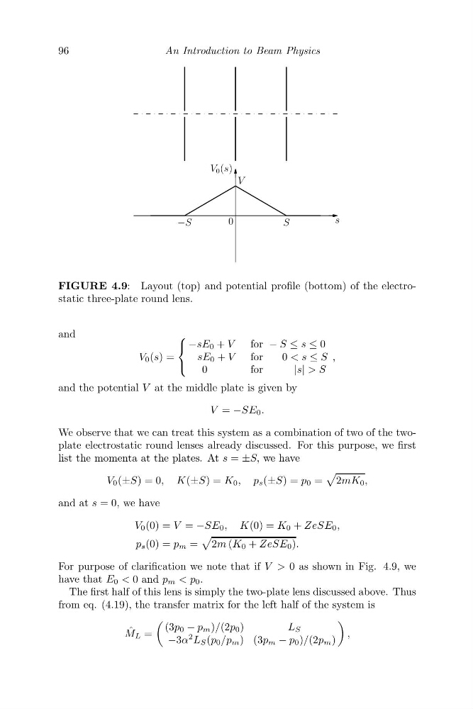
FIGURE 4.9: Layout (top) and potential profile (bottom) of the electrostatic three-plate round lens.
and
V 0 (s) =
⎧
⎨
⎩
−sE 0 + V
for − S ≤ s ≤ 0
sE 0 + V
for
0 < s ≤ S
0
f o r
|s| > S
,
and the potential V at the middle plate is given by
V = −SE 0 .
We observe that we can treat this system as a combination of two of the twoplate electrostatic round lenses already discussed. For this purpose, we first
list the momenta at the plates. At s = ±S, we have
V 0 (±S) = 0, K(±S) = K 0 , p s (±S) = p 0 =
2mK 0 ,
and at s = 0, we have
V 0 (0) = V = −SE 0 , K(0) = K 0 + ZeSE 0 ,
p s (0) = p m =
2m (K 0 + ZeSE 0 ).
For purpose of clarification we note that if V > 0 as shown in Fig. 4.9, we
have that E 0 < 0 and p m < p 0 .
The first half of this lens is simply the two-plate lens discussed above. Thus
from eq. (4.19), the transfer matrix for the left half of the system is
ˆ
M L =
(3p 0 − p m )/(2p 0 )
L S
−3α
2 L S (p 0 /p m ) (3p m − p 0 )/(2p m )
,
An Introduction to Beam Physics
V 0 (s)
s
V
−S
S
0
FIGURE 4.9: Layout (top) and potential profile (bottom) of the electrostatic three-plate round lens.
and
V 0 (s) =
⎧
⎨
⎩
−sE 0 + V
for − S ≤ s ≤ 0
sE 0 + V
for
0 < s ≤ S
0
f o r
|s| > S
,
and the potential V at the middle plate is given by
V = −SE 0 .
We observe that we can treat this system as a combination of two of the twoplate electrostatic round lenses already discussed. For this purpose, we first
list the momenta at the plates. At s = ±S, we have
V 0 (±S) = 0, K(±S) = K 0 , p s (±S) = p 0 =
2mK 0 ,
and at s = 0, we have
V 0 (0) = V = −SE 0 , K(0) = K 0 + ZeSE 0 ,
p s (0) = p m =
2m (K 0 + ZeSE 0 ).
For purpose of clarification we note that if V > 0 as shown in Fig. 4.9, we
have that E 0 < 0 and p m < p 0 .
The first half of this lens is simply the two-plate lens discussed above. Thus
from eq. (4.19), the transfer matrix for the left half of the system is
ˆ
M L =
(3p 0 − p m )/(2p 0 )
L S
−3α
2 L S (p 0 /p m ) (3p m − p 0 )/(2p m )
,