

�[
]
(
)�
�
�
Applying BC (i) into Equation 3.26,
∞
q s = −k
C n λ n cosh (λ n x) − coth (λ n a) λ n sinh (λ n x) cos λ n y x=0
n=1
∞
(
)
q s = −k
C n λ n cos λ n y
n=1
b
cos
(
)
λ n y dy =
b
�
0
C n cos 2 ( λ n y
)
dy
−
q s
k λ n
0
�
(
)
(
) � b
q s 1
(
)�
y
2 sin λ n y cos λ n y
−
sin λ n y
b = C n
+
0
k λ n λ n
2
4λ n
0
(
)
2q s sin λ n b
C n = −
( (
)
(
)
)
k λ n sin λ n b cos λ n b + bλ n
(
)
∞
2q s sin λ n b
θ =
( (
)
(
)
)
k λ n sin λ n b cos λ n b + bλ n
n=1
[
]
(
)
× − sinh (λ n x) + coth (λ n a) cosh (λ n x) cos λ n y
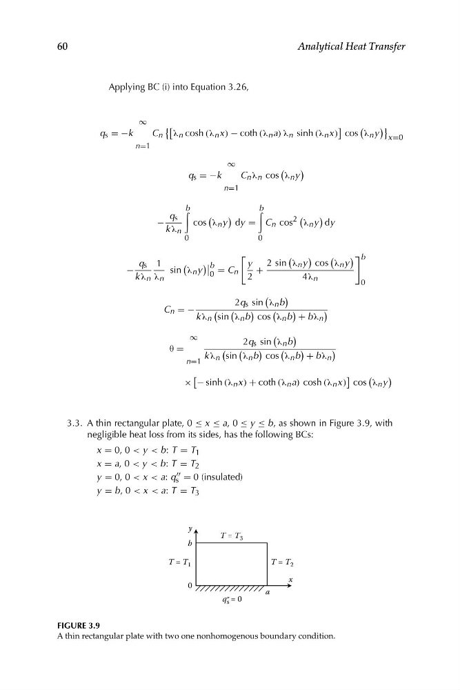
3.3. A thin rectangular plate, 0 ≤ x ≤ a, 0 ≤ y ≤ b, as shown in Figure 3.9, with
negligible heat loss from its sides, has the following BCs:
x = 0, 0 < y < b: T = T 1
x = a, 0 < y < b: T = T 2
""
y = 0, 0 < x < a: q = 0 (insulated)
s
y b, 0 < x < a: T T 3
=
=
x
y
b
0
T = T 3
T = T 1
T = T 2
a
q″ = 0
s
60
Analytical Heat Transfer
FIGURE 3.9
A thin rectangular plate with two one nonhomogenous boundary condition.
]
(
)�
�
�
Applying BC (i) into Equation 3.26,
∞
q s = −k
C n λ n cosh (λ n x) − coth (λ n a) λ n sinh (λ n x) cos λ n y x=0
n=1
∞
(
)
q s = −k
C n λ n cos λ n y
n=1
b
cos
(
)
λ n y dy =
b
�
0
C n cos 2 ( λ n y
)
dy
−
q s
k λ n
0
�
(
)
(
) � b
q s 1
(
)�
y
2 sin λ n y cos λ n y
−
sin λ n y
b = C n
+
0
k λ n λ n
2
4λ n
0
(
)
2q s sin λ n b
C n = −
( (
)
(
)
)
k λ n sin λ n b cos λ n b + bλ n
(
)
∞
2q s sin λ n b
θ =
( (
)
(
)
)
k λ n sin λ n b cos λ n b + bλ n
n=1
[
]
(
)
× − sinh (λ n x) + coth (λ n a) cosh (λ n x) cos λ n y
3.3. A thin rectangular plate, 0 ≤ x ≤ a, 0 ≤ y ≤ b, as shown in Figure 3.9, with
negligible heat loss from its sides, has the following BCs:
x = 0, 0 < y < b: T = T 1
x = a, 0 < y < b: T = T 2
""
y = 0, 0 < x < a: q = 0 (insulated)
s
y b, 0 < x < a: T T 3
=
=
x
y
b
0
T = T 3
T = T 1
T = T 2
a
q″ = 0
s
60
Analytical Heat Transfer
FIGURE 3.9
A thin rectangular plate with two one nonhomogenous boundary condition.