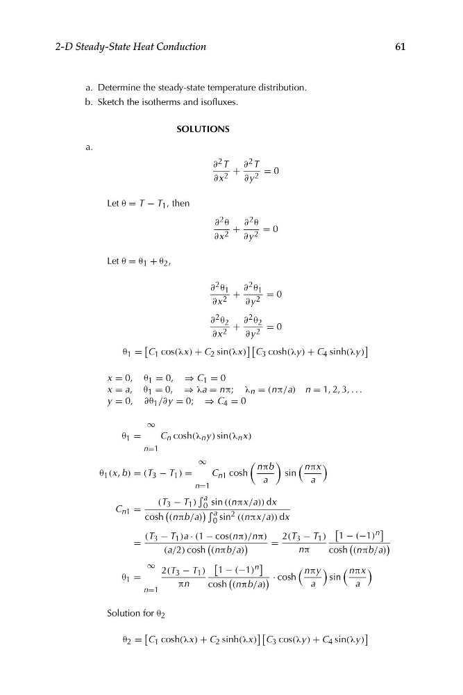
�
�
�
a. Determine the steady-state temperature distribution.
b. Sketch the isotherms and isofluxes.
SOLUTIONS
a.
∂ 2 T
∂ 2 T
+
= 0
∂x 2
∂y 2
Let θ = T − T 1 , then
∂ 2 θ
∂ 2 θ
+
= 0
∂x 2
∂y 2
Let θ = θ 1 + θ 2 ,
∂ 2 θ 1
∂ 2 θ 1
+
= 0
∂x 2
∂y 2
∂ 2 θ 2
∂ 2 θ 2
+
= 0
∂x 2
∂y 2
[
] [
]
θ 1 = C 1 cos(λx) + C 2 sin(λx) C 3 cosh(λy ) + C 4 sinh(λy )
x = 0, θ 1 = 0, ⇒ C 1 = 0
x = a, θ 1 = 0, ⇒ λa = nπ; λ n = (nπ/a) n = 1, 2, 3, . . .
y = 0, ∂θ 1 /∂y = 0; ⇒ C 4 = 0
∞
θ 1 =
C n cosh(λ n y ) sin(λ n x)

n=1

∞
(
)
nπb
nπx
θ 1 (x, b) = (T 3 − T 1 ) =
C n1 cosh
sin
a
a
n=1
a
(T 3 − T 1 ) 0 sin ((nπx/a)) dx
C n1 =
(
) � a
cosh (nπb/a) 0 sin 2 ((nπx/a)) dx
[
]
(T 3 − T 1 )a · (1 − cos(nπ)/nπ)
2(T 3 − T 1 ) 1 − (−1) n
=
(
)
=
(
)
(a/2) cosh (nπb/a)
nπ
cosh (nπb/a)
∞
[
]
(
)
(
)
2(T 3 − T 1 ) 1 − (−1) n
nπy
nπx
θ 1 =
(
) · cosh
sin
πn
cosh (nπb/a)
a
a
n=1
Solution for θ 2
[
] [
]
θ 2 = C 1 cosh(λx) + C 2 sinh(λx) C 3 cos(λy ) + C 4 sin(λy )
61
2-D Steady-State Heat Conduction