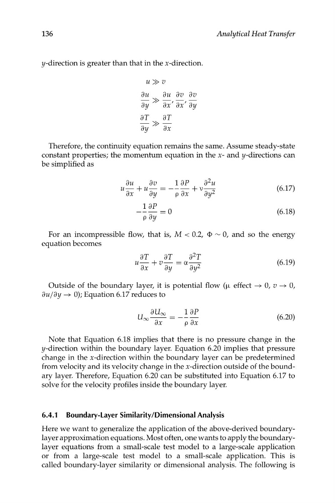
y-direction is greater than that in the x-direction.
u » v
∂u
∂u ∂v ∂v
»
, ,
∂y
∂x ∂x ∂y
∂T
∂T
»
∂y
∂x
Therefore, the continuity equation remains the same. Assume steady-state
constant properties; the momentum equation in the x- and y-directions can
be simplified as
∂u
∂v
1 ∂P
∂ 2 u
u
+ u
= −
+ ν
(6.17)
∂x
∂y
ρ ∂x
∂y 2
1 ∂P
−
= 0
(6.18)
ρ ∂y
For an incompressible flow, that is, M < 0.2, Φ ∼ 0, and so the energy
equation becomes
∂T
∂T
∂ 2 T
u
+ v
= α
(6.19)
∂x
∂y
∂y 2
Outside of the boundary layer, it is potential flow (μ effect → 0, v → 0,
∂u/∂y → 0); Equation 6.17 reduces to
∂U ∞
1 ∂P
U ∞
= −
(6.20)
∂x
ρ ∂x
136
Analytical Heat Transfer
Note that Equation 6.18 implies that there is no pressure change in the
y-direction within the boundary layer. Equation 6.20 implies that pressure
change in the x-direction within the boundary layer can be predetermined
from velocity and its velocity change in the x-direction outside of the boundary layer. Therefore, Equation 6.20 can be substituted into Equation 6.17 to
solve for the velocity profiles inside the boundary layer.
6.4.1 Boundary-Layer Similarity/Dimensional Analysis
Here we want to generalize the application of the above-derived boundarylayer approximation equations. Most often, one wants to apply the boundarylayer equations from a small-scale test model to a large-scale application
or from a large-scale test model to a small-scale application. This is
called boundary-layer similarity or dimensional analysis. The following is