

�
�
�
�
�
�
92
Analytical Heat Transfer
(3) after the steady-state ablation velocity has been reached, the temperature
distribution in the material is steady. The initial transient problem has been
solved before (i.e., V a = 0, given the surface heat flux BC). The second transient problem, Equation 4.38, can be solved by the finite-difference method.
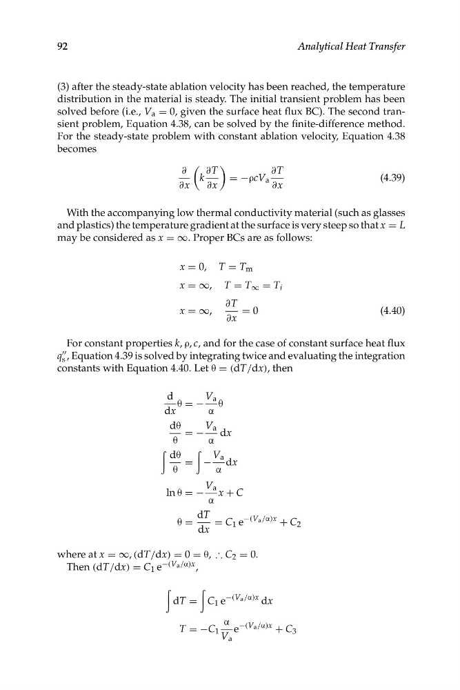
For the steady-state problem with constant ablation velocity, Equation 4.38
becomes
∂
∂T
∂T
k
= −ρcV a
(4.39)
∂x
∂x
∂x
With the accompanying low thermal conductivity material (such as glasses
and plastics) the temperature gradient at the surface is very steep so that x = L
may be considered as x = ∞. Proper BCs are as follows:
x = 0, T = T m
x = ∞, T = T ∞ = T i
∂T
x = ∞,
= 0
(4.40)
∂x
For constant properties k, ρ, c, and for the case of constant surface heat flux
""
q , Equation 4.39 is solved by integrating twice and evaluating the integration
s
constants with Equation 4.40. Let θ = (dT/dx), then
d
V a
θ = − θ
dx
α
dθ
V a
= −
dx
θ
α
dθ
V a
= − dx
θ
α
V a
ln θ = − x + C
α
θ =
dT = C 1 e
−(V a /α)x
+ C 2
dx
where at x = ∞, (dT/dx) = 0 = θ, ∴ C 2 = 0.
−(V a /α)x
Then (dT/dx) = C 1 e
,
−(V a /α)x dx
dT = C 1 e
α
T = −C 1 e
−(V a /α)x
+ C 3
V a
�
�
�
�
�
92
Analytical Heat Transfer
(3) after the steady-state ablation velocity has been reached, the temperature
distribution in the material is steady. The initial transient problem has been
solved before (i.e., V a = 0, given the surface heat flux BC). The second transient problem, Equation 4.38, can be solved by the finite-difference method.
For the steady-state problem with constant ablation velocity, Equation 4.38
becomes
∂
∂T
∂T
k
= −ρcV a
(4.39)
∂x
∂x
∂x
With the accompanying low thermal conductivity material (such as glasses
and plastics) the temperature gradient at the surface is very steep so that x = L
may be considered as x = ∞. Proper BCs are as follows:
x = 0, T = T m
x = ∞, T = T ∞ = T i
∂T
x = ∞,
= 0
(4.40)
∂x
For constant properties k, ρ, c, and for the case of constant surface heat flux
""
q , Equation 4.39 is solved by integrating twice and evaluating the integration
s
constants with Equation 4.40. Let θ = (dT/dx), then
d
V a
θ = − θ
dx
α
dθ
V a
= −
dx
θ
α
dθ
V a
= − dx
θ
α
V a
ln θ = − x + C
α
θ =
dT = C 1 e
−(V a /α)x
+ C 2
dx
where at x = ∞, (dT/dx) = 0 = θ, ∴ C 2 = 0.
−(V a /α)x
Then (dT/dx) = C 1 e
,
−(V a /α)x dx
dT = C 1 e
α
T = −C 1 e
−(V a /α)x
+ C 3
V a