

q s ″
T ∞
T m
V a
T i = T ∞
x = 0
x = L, ∞
�
�
91
Transient Heat Conduction
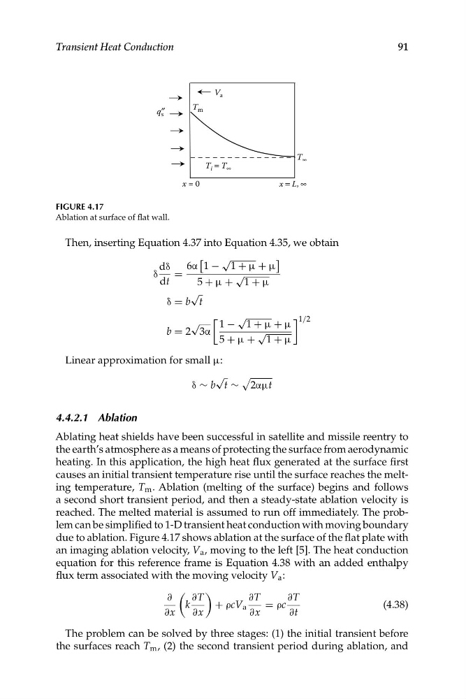
FIGURE 4.17
Ablation at surface of flat wall.
Then, inserting Equation 4.37 into Equation 4.35, we obtain
[
√
]
dδ
6α 1 − 1 + μ + μ
δ
=
√
dt
5 + μ + 1 + μ
√
δ = b t
�
√
� 1/2
√
1 − 1 + μ + μ
b = 2 3α
√
5 + μ + 1 + μ
Linear approximation for small μ:
√
)
δ ∼ b t ∼ 2αμt
4.4.2.1 Ablation
Ablating heat shields have been successful in satellite and missile reentry to
the earth’s atmosphere as a means of protecting the surface from aerodynamic
heating. In this application, the high heat flux generated at the surface first
causes an initial transient temperature rise until the surface reaches the melting temperature, T m . Ablation (melting of the surface) begins and follows
a second short transient period, and then a steady-state ablation velocity is
reached. The melted material is assumed to run off immediately. The problem can be simplified to 1-D transient heat conduction with moving boundary
due to ablation. Figure 4.17 shows ablation at the surface of the flat plate with
an imaging ablation velocity, V a , moving to the left [5]. The heat conduction
equation for this reference frame is Equation 4.38 with an added enthalpy
flux term associated with the moving velocity V a :
∂
∂T
∂T
∂T
k
+ ρcV a
= ρc
(4.38)
∂x
∂x
∂x
∂t
The problem can be solved by three stages: (1) the initial transient before
the surfaces reach T m , (2) the second transient period during ablation, and
T ∞
T m
V a
T i = T ∞
x = 0
x = L, ∞
�
�
91
Transient Heat Conduction
FIGURE 4.17
Ablation at surface of flat wall.
Then, inserting Equation 4.37 into Equation 4.35, we obtain
[
√
]
dδ
6α 1 − 1 + μ + μ
δ
=
√
dt
5 + μ + 1 + μ
√
δ = b t
�
√
� 1/2
√
1 − 1 + μ + μ
b = 2 3α
√
5 + μ + 1 + μ
Linear approximation for small μ:
√
)
δ ∼ b t ∼ 2αμt
4.4.2.1 Ablation
Ablating heat shields have been successful in satellite and missile reentry to
the earth’s atmosphere as a means of protecting the surface from aerodynamic
heating. In this application, the high heat flux generated at the surface first
causes an initial transient temperature rise until the surface reaches the melting temperature, T m . Ablation (melting of the surface) begins and follows
a second short transient period, and then a steady-state ablation velocity is
reached. The melted material is assumed to run off immediately. The problem can be simplified to 1-D transient heat conduction with moving boundary
due to ablation. Figure 4.17 shows ablation at the surface of the flat plate with
an imaging ablation velocity, V a , moving to the left [5]. The heat conduction
equation for this reference frame is Equation 4.38 with an added enthalpy
flux term associated with the moving velocity V a :
∂
∂T
∂T
∂T
k
+ ρcV a
= ρc
(4.38)
∂x
∂x
∂x
∂t
The problem can be solved by three stages: (1) the initial transient before
the surfaces reach T m , (2) the second transient period during ablation, and