

205
Interaction of Extremely Low–Frequency Electromagnetic Fields
∑
6
⎛
6
⎞
s n ϕ n − ⎜ s
⎝
∑ n ϕ =
⎟
jω
⎠
0
∑
6 6
(−1)
n
s n λ n A 0n
(4.8)
n=1
n=1
n=1
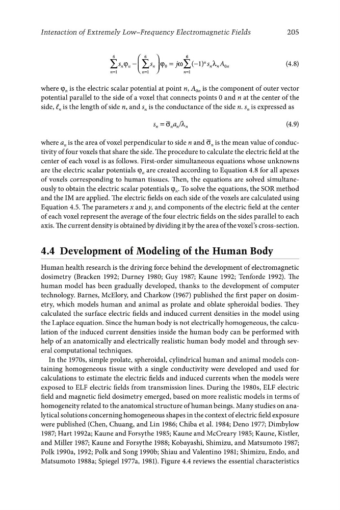
where φ n is the electric scalar potential at point n, A 0n is the component of outer vector
potential parallel to the side of a voxel that connects points 0 and n at the center of the
side, ℓ n is the length of side n, and s n is the conductance of the side n. s n is expressed as
s n = σ n a n /λ n
(4.9)
where a n is the area of voxel perpendicular to side n and σ n is the mean value of conductivity of four voxels that share the side. The procedure to calculate the electric field at the
center of each voxel is as follows. First-order simultaneous equations whose unknowns
are the electric scalar potentials φ n are created according to Equation 4.8 for all apexes
of voxels corresponding to human tissues. Then, the equations are solved simultaneously to obtain the electric scalar potentials φ n . To solve the equations, the SOR method
and the IM are applied. The electric fields on each side of the voxels are calculated using
Equation 4.5. The parameters x and y, and components of the electric field at the center
of each voxel represent the average of the four electric fi elds on the sides parallel to e ach
axis. The current density is obtained by dividing it by the area of the voxel’s cross-section.
4.4 Development of Modeling of the Human Body
Human health research is the driving force behind the development of electromagnetic
dosimetry (Bracken 1992; Durney 1980; Guy 1987; Kaune 1992; Tenforde 1992). The
human model has been gradually developed, thanks to the development of computer
technology. Barnes, McElory, and Charkow (1967) published the first paper on dosimetry, which models human and animal as prolate and oblate spheroidal bodies. They
calculated the surface electric fields and induced current densities in the model using
the Laplace equation. Since the human body is not electrically homogeneous, the calculation of the induced current densities inside the human body can be performed with
help of an anatomically and electrically realistic human body model and through several computational techniques.
In the 1970s, simple prolate, spheroidal, cylindrical human and animal models containing homogeneous tissue with a single conductivity were developed and used for
calculations to estimate the electric fields and induced currents when the models were
exposed to ELF electric fields from transmission lines. During the 1980s, ELF electric
field and magnetic field dosimetry emerged, based on more realistic models in terms of
homogeneity related to the anatomical structure of human beings. Many studies on analytical solutions concerning homogeneous shapes in the context of electric field exposure
were published (Chen, Chuang, and Lin 1986; Chiba et al. 1984; Deno 1977; Dimbylow
1987; Hart 1992a; Kaune and Forsythe 1985; Kaune and McCreary 1985; Kaune, Kistler,
and Miller 1987; Kaune and Forsythe 1988; Kobayashi, Shimizu, and Matsumoto 1987;
Polk 1990a, 1992; Polk and Song 1990b; Shiau and Valentino 1981; Shimizu, Endo, and
Matsumoto 1988a; Spiegel 1977a, 1981). Figure 4.4 reviews the essential characteristics
Interaction of Extremely Low–Frequency Electromagnetic Fields
∑
6
⎛
6
⎞
s n ϕ n − ⎜ s
⎝
∑ n ϕ =
⎟
jω
⎠
0
∑
6 6
(−1)
n
s n λ n A 0n
(4.8)
n=1
n=1
n=1
where φ n is the electric scalar potential at point n, A 0n is the component of outer vector
potential parallel to the side of a voxel that connects points 0 and n at the center of the
side, ℓ n is the length of side n, and s n is the conductance of the side n. s n is expressed as
s n = σ n a n /λ n
(4.9)
where a n is the area of voxel perpendicular to side n and σ n is the mean value of conductivity of four voxels that share the side. The procedure to calculate the electric field at the
center of each voxel is as follows. First-order simultaneous equations whose unknowns
are the electric scalar potentials φ n are created according to Equation 4.8 for all apexes
of voxels corresponding to human tissues. Then, the equations are solved simultaneously to obtain the electric scalar potentials φ n . To solve the equations, the SOR method
and the IM are applied. The electric fields on each side of the voxels are calculated using
Equation 4.5. The parameters x and y, and components of the electric field at the center
of each voxel represent the average of the four electric fi elds on the sides parallel to e ach
axis. The current density is obtained by dividing it by the area of the voxel’s cross-section.
4.4 Development of Modeling of the Human Body
Human health research is the driving force behind the development of electromagnetic
dosimetry (Bracken 1992; Durney 1980; Guy 1987; Kaune 1992; Tenforde 1992). The
human model has been gradually developed, thanks to the development of computer
technology. Barnes, McElory, and Charkow (1967) published the first paper on dosimetry, which models human and animal as prolate and oblate spheroidal bodies. They
calculated the surface electric fields and induced current densities in the model using
the Laplace equation. Since the human body is not electrically homogeneous, the calculation of the induced current densities inside the human body can be performed with
help of an anatomically and electrically realistic human body model and through several computational techniques.
In the 1970s, simple prolate, spheroidal, cylindrical human and animal models containing homogeneous tissue with a single conductivity were developed and used for
calculations to estimate the electric fields and induced currents when the models were
exposed to ELF electric fields from transmission lines. During the 1980s, ELF electric
field and magnetic field dosimetry emerged, based on more realistic models in terms of
homogeneity related to the anatomical structure of human beings. Many studies on analytical solutions concerning homogeneous shapes in the context of electric field exposure
were published (Chen, Chuang, and Lin 1986; Chiba et al. 1984; Deno 1977; Dimbylow
1987; Hart 1992a; Kaune and Forsythe 1985; Kaune and McCreary 1985; Kaune, Kistler,
and Miller 1987; Kaune and Forsythe 1988; Kobayashi, Shimizu, and Matsumoto 1987;
Polk 1990a, 1992; Polk and Song 1990b; Shiau and Valentino 1981; Shimizu, Endo, and
Matsumoto 1988a; Spiegel 1977a, 1981). Figure 4.4 reviews the essential characteristics