

104
Electromagnetic Fields in Biological Systems
An additional utility of such dielectric parameter measurements is in medical diagnostics. This is linked to the fact that electrical properties (e.g., permittivity and conductivity) of cells and tissues are distinct for each type. This occurs due to variability in
moisture content, size, distributions of molecular dipole moments, density, and texture
(Gabriel, Lau, and Gabriel 1996). For example, fat has a lower permittivity and conductivity than muscle. Even for the same tissue, a pathological change may result in
different electric properties (Semenov et al. 2002). Hence, electrical properties can be
used not only to differentiate the anatomical structure but also to differentially diagnose
malignant versus normal tissue, providing “functional” information.
Another application can be toward real-time monitoring of treatment responses. For
example, high-field electric pulsing can lead to nonlinear cell membrane effects such as
electroporation (Schoenbach et al. 2004). This alters the effective conductivity of cells
and allows the passage of molecules (including drugs and chemotherapeutic agents) into
cells. Loading molecules into cells should then result in a strong contrast of conductivity within the tissue. In practice, four types of cells could exist in such treated tissue: normal, malignant, normal loaded with delivered molecules, and malignant cells
loaded with delivered molecules. The average dielectric properties of the tissues should
be different depending on the percentage compositions of the four cell types in the tissue. Presumably, tissue with a dominant percentage of tumor cells should have a higher
dielectric permittivity than the tissue in which normal cells dominate. Such difference
can be 10% to 10-fold depending on the tissue composition (Lazebnik et al. 2007). The
drug-loaded tissue should have a dielectric permittivity in between this range. Hence,
the dielectric properties can be a good marker to monitor targeted drug delivery and
to ascertain whether the agents introduced do indeed have the intended consequence
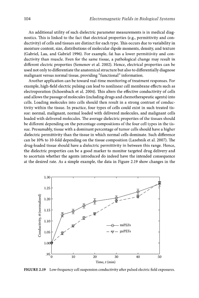
at the desired rate. As a simple example, the data in Figure 2.19 show changes in the
1.30
1.25
1.20
1.15
1.10
1.05
.95 0
10
20
30
50
Time, t (min)
Conductivity, σ
(normalized)
40
nsPEFs
μsPEFs
1.00
Figure 2.19 Low-frequency cell suspension conductivity after pulsed electric field exposures.
Electromagnetic Fields in Biological Systems
An additional utility of such dielectric parameter measurements is in medical diagnostics. This is linked to the fact that electrical properties (e.g., permittivity and conductivity) of cells and tissues are distinct for each type. This occurs due to variability in
moisture content, size, distributions of molecular dipole moments, density, and texture
(Gabriel, Lau, and Gabriel 1996). For example, fat has a lower permittivity and conductivity than muscle. Even for the same tissue, a pathological change may result in
different electric properties (Semenov et al. 2002). Hence, electrical properties can be
used not only to differentiate the anatomical structure but also to differentially diagnose
malignant versus normal tissue, providing “functional” information.
Another application can be toward real-time monitoring of treatment responses. For
example, high-field electric pulsing can lead to nonlinear cell membrane effects such as
electroporation (Schoenbach et al. 2004). This alters the effective conductivity of cells
and allows the passage of molecules (including drugs and chemotherapeutic agents) into
cells. Loading molecules into cells should then result in a strong contrast of conductivity within the tissue. In practice, four types of cells could exist in such treated tissue: normal, malignant, normal loaded with delivered molecules, and malignant cells
loaded with delivered molecules. The average dielectric properties of the tissues should
be different depending on the percentage compositions of the four cell types in the tissue. Presumably, tissue with a dominant percentage of tumor cells should have a higher
dielectric permittivity than the tissue in which normal cells dominate. Such difference
can be 10% to 10-fold depending on the tissue composition (Lazebnik et al. 2007). The
drug-loaded tissue should have a dielectric permittivity in between this range. Hence,
the dielectric properties can be a good marker to monitor targeted drug delivery and
to ascertain whether the agents introduced do indeed have the intended consequence
at the desired rate. As a simple example, the data in Figure 2.19 show changes in the
1.30
1.25
1.20
1.15
1.10
1.05
.95 0
10
20
30
50
Time, t (min)
Conductivity, σ
(normalized)
40
nsPEFs
μsPEFs
1.00
Figure 2.19 Low-frequency cell suspension conductivity after pulsed electric field exposures.