156
Relic neutrinos and axions
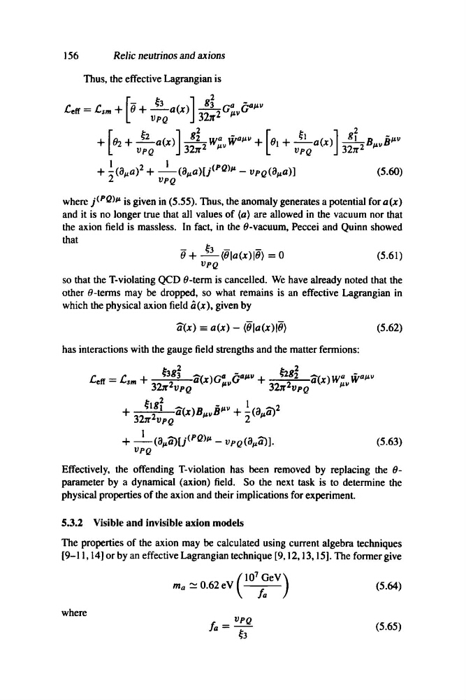
Thus, the effective Lagrangian is
[ -0
~3 ()] g~ Ga G-a/J.II
C
C
eff = 11/11 + + vPQ a x 321r2 /J.II
+ [fh + ~a(x)] g~ Wall W a /J.II + [01 + l!....a(x)] ~B/J.llj/J.II
VPQ
321r 2 /J.
vPQ
3211'2
+ -2 1 (a/J.a)2 + _1_(a/J.a)[j(PQ)/J. - vPQ(a/J.a»)
(S.60)
vPQ
where j and it is no longer true that all values of (a) are allowed in the vacuum nor that
the axion field is massless. In fact. in the O-vacuum. Peccei and Quinn showed
that
o + ~(Ola(x)IO) = 0
(5.61)
uPQ
so that the T-violating QCD 9-term is cancelled. We have already noted that the
other 9-terms may be dropped, so what remains is an effective Lagrangian in
which the physical axion field a(x), given by
a(x) = a(x) - (Ola(x)IO)
(5.62)
has interactions with the gauge field strengths and the matter fermions:
C = C + ~3g~ ..... ( )GII G-a/J.II + bg~ ..... ( )Wa W-a/J.II
eff
11/11
3"-2
a x 1-'"
3"-2
a x /J.II
~, VPQ
~ VPQ
~lgf ..... ()B -1-'11 I (a ~2
+ 321r2vpQ a x /J.IIB + ' 2 /J.a}
+ _1_(al-'Q)[j (S.63)
vPQ
Effectively, the offending T-violation has been removed by replacing the 0parameter by a dynamical (axion) field. So the next task is to determine the
physical properties of the axion and their implications for experiment.
5.3.2 Visible and invisible axion models
The properties of the axion may be calculated using current algebra techniques
[9-11,14] or by an effective Lagrangian technique [9.12, 13,15]. The former give
ma ~ 0.62 eV (107f~V)
(5.64)
where
fa = vPQ
(5.6S)
~3