

470
P. Grassmann Variables
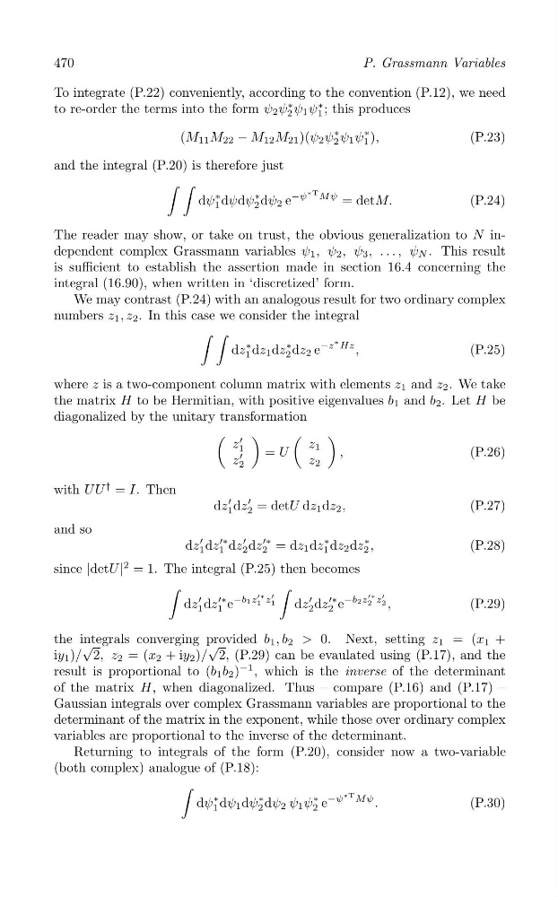
To integrate (P.22) conveniently, according to the convention (P.12), we need
to re-order the terms into the form ψ 2 ψ 2
∗ ψ 1 ψ 1
∗ ; this produces
(M 11 M 22 − M 12 M 21 )(ψ 2 ψ 2
∗ ψ 1 ψ 1
∗ ),
(P.23)
and the integral (P.20) is therefore just
∫ ∫
∗
dψ 1
∗ dψdψ 2
∗ dψ 2 e
−ψ
T Mψ = detM.
(P.24)
The reader may show, or take on trust, the obvious generalization to N independent complex Grassmann variables ψ 1 , ψ 2 , ψ 3 , . . . , ψ N . This result
is sufficient to establish the assertion made in section 16.4 concerning the
integral (16.90), when written in ‘discretized’ form.
We may contrast (P.24) with an analogous result for two ordinary complex
numbers z 1 , z 2 . In this case we consider the integral
∫ ∫
dz 1
∗ dz 1 dz 2
∗
∗
dz 2 e
−z Hz ,
(P.25)
where z is a two-component column matrix with elements z 1 and z 2 . We take
the matrix H to be Hermitian, with positive eigenvalues b 1 and b 2 . Let H be
diagonalized by the unitary transformation
(
)
(
)
z 1
′
z
= U
1
,
(P.26)
z 2
′
z 2
with U U
† = I. Then
dz 1
′ dz 2
′ = detU dz 1 dz 2 ,
(P.27)
and so
dz 1
′ dz 1
′∗ dz 2
′ dz 2
′∗ = dz 1 dz 1
∗ dz 2 dz 2
∗ ,
(P.28)
since |detU |
2 = 1. The integral (P.25) then becomes
∫
∫
′
′∗ −b1z 1
′∗ z 1
′
′
′∗ −b2z 2
′∗ ′
dz dz e
dz dz e
z 2
1
1
2
2
,
(P.29)
the i √ ntegrals converging provided b 1 , b 2 > 0. Next, setting z 1 = (x 1 +
iy 1 )/ 2, z 2 = (x 2 + iy 2 )/
√
2, (P.29) can be evaulated using (P.17), and the
result is proportional to (b 1 b
1
2 )
− , which is the inverse of the determinant
of the matrix H, when diagonalized. Thus – compare (P.16) and (P.17) –
Gaussian integrals over complex Grassmann variables are proportional to the
determinant of the matrix in the exponent, while those over ordinary complex
variables are proportional to the inverse of the determinant.
Returning to integrals of the form (P.20), consider now a two-variable
(both complex) analogue of (P.18):
∫
dψ 1
∗ dψ 1 dψ 2
∗
∗T
dψ 2 ψ ψ 2
∗ e
−ψ Mψ
1
.
(P.30)
P. Grassmann Variables
To integrate (P.22) conveniently, according to the convention (P.12), we need
to re-order the terms into the form ψ 2 ψ 2
∗ ψ 1 ψ 1
∗ ; this produces
(M 11 M 22 − M 12 M 21 )(ψ 2 ψ 2
∗ ψ 1 ψ 1
∗ ),
(P.23)
and the integral (P.20) is therefore just
∫ ∫
∗
dψ 1
∗ dψdψ 2
∗ dψ 2 e
−ψ
T Mψ = detM.
(P.24)
The reader may show, or take on trust, the obvious generalization to N independent complex Grassmann variables ψ 1 , ψ 2 , ψ 3 , . . . , ψ N . This result
is sufficient to establish the assertion made in section 16.4 concerning the
integral (16.90), when written in ‘discretized’ form.
We may contrast (P.24) with an analogous result for two ordinary complex
numbers z 1 , z 2 . In this case we consider the integral
∫ ∫
dz 1
∗ dz 1 dz 2
∗
∗
dz 2 e
−z Hz ,
(P.25)
where z is a two-component column matrix with elements z 1 and z 2 . We take
the matrix H to be Hermitian, with positive eigenvalues b 1 and b 2 . Let H be
diagonalized by the unitary transformation
(
)
(
)
z 1
′
z
= U
1
,
(P.26)
z 2
′
z 2
with U U
† = I. Then
dz 1
′ dz 2
′ = detU dz 1 dz 2 ,
(P.27)
and so
dz 1
′ dz 1
′∗ dz 2
′ dz 2
′∗ = dz 1 dz 1
∗ dz 2 dz 2
∗ ,
(P.28)
since |detU |
2 = 1. The integral (P.25) then becomes
∫
∫
′
′∗ −b1z 1
′∗ z 1
′
′
′∗ −b2z 2
′∗ ′
dz dz e
dz dz e
z 2
1
1
2
2
,
(P.29)
the i √ ntegrals converging provided b 1 , b 2 > 0. Next, setting z 1 = (x 1 +
iy 1 )/ 2, z 2 = (x 2 + iy 2 )/
√
2, (P.29) can be evaulated using (P.17), and the
result is proportional to (b 1 b
1
2 )
− , which is the inverse of the determinant
of the matrix H, when diagonalized. Thus – compare (P.16) and (P.17) –
Gaussian integrals over complex Grassmann variables are proportional to the
determinant of the matrix in the exponent, while those over ordinary complex
variables are proportional to the inverse of the determinant.
Returning to integrals of the form (P.20), consider now a two-variable
(both complex) analogue of (P.18):
∫
dψ 1
∗ dψ 1 dψ 2
∗
∗T
dψ 2 ψ ψ 2
∗ e
−ψ Mψ
1
.
(P.30)