

P. Grassmann Variables
469
It is convenient to define complex conjugation to include reversing the order
of quantities:
(ψχ)
∗ = χ
∗ ψ
∗ .
(P.15)
Then (P.14) is consistent under complex conjugation.
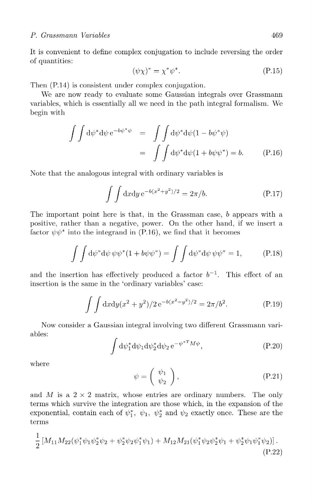
We are now ready to evaluate some Gaussian integrals over Grassmann
variables, which is essentially all we need in the path integral formalism. We
begin with
∫ ∫
∫ ∫
dψ
∗ dψ e
−bψ
∗ ψ
=
dψ
∗ dψ(1 − bψ
∗ ψ)
∫ ∫
=
dψ
∗ dψ(1 + bψψ
∗ ) = b.
(P.16)
Note that the analogous integral with ordinary variables is
∫ ∫
dxdy e
−b(x
2 +y
2 )/2 = 2π/b.
(P.17)
The important point here is that, in the Grassman case, b appears with a
positive, rather than a negative, power. On the other hand, if we insert a
factor ψψ
∗ into the integrand in (P.16), we find that it becomes
∫ ∫
∫ ∫
dψ
∗ dψ ψψ
∗ (1 + bψψ
∗ ) =
dψ
∗ dψ ψψ
∗ = 1,
(P.18)
and the insertion has effectively produced a factor b
−1 . This effect of an
insertion is the same in the ‘ordinary variables’ case:
∫ ∫
dxdy(x
2 + y
2 )/2 e
−b(x
2 +y
2 )/2 = 2π/b
2 .
(P.19)
Now consider a Gaussian integral involving two different Grassmann variables:
∫
dψ 1
∗
∗
dψ
ψ
T Mψ
1 dψ 2
∗ dψ 2 e
−
,
(P.20)
where
(
)
ψ
ψ =
1
,
(P.21)
ψ 2
and M is a 2 × 2 matrix, whose entries are ordinary numbers. The only
terms which survive the integration are those which, in the expansion of the
exponential, contain each of ψ 1
∗ , ψ 1 , ψ 2
∗ and ψ 2 exactly once. These are the
terms
1 [M 11 M 22 (ψ
∗
2
1 ψ 1 ψ 2
∗ ψ 2 + ψ 2
∗ ψ 2 ψ 1
∗ ψ 1 ) + M 12 M 21 (ψ 1
∗ ψ 2 ψ 2
∗ ψ 1 + ψ 2
∗ ψ 1 ψ 1
∗ ψ 2 )] .
(P.22)
469
It is convenient to define complex conjugation to include reversing the order
of quantities:
(ψχ)
∗ = χ
∗ ψ
∗ .
(P.15)
Then (P.14) is consistent under complex conjugation.
We are now ready to evaluate some Gaussian integrals over Grassmann
variables, which is essentially all we need in the path integral formalism. We
begin with
∫ ∫
∫ ∫
dψ
∗ dψ e
−bψ
∗ ψ
=
dψ
∗ dψ(1 − bψ
∗ ψ)
∫ ∫
=
dψ
∗ dψ(1 + bψψ
∗ ) = b.
(P.16)
Note that the analogous integral with ordinary variables is
∫ ∫
dxdy e
−b(x
2 +y
2 )/2 = 2π/b.
(P.17)
The important point here is that, in the Grassman case, b appears with a
positive, rather than a negative, power. On the other hand, if we insert a
factor ψψ
∗ into the integrand in (P.16), we find that it becomes
∫ ∫
∫ ∫
dψ
∗ dψ ψψ
∗ (1 + bψψ
∗ ) =
dψ
∗ dψ ψψ
∗ = 1,
(P.18)
and the insertion has effectively produced a factor b
−1 . This effect of an
insertion is the same in the ‘ordinary variables’ case:
∫ ∫
dxdy(x
2 + y
2 )/2 e
−b(x
2 +y
2 )/2 = 2π/b
2 .
(P.19)
Now consider a Gaussian integral involving two different Grassmann variables:
∫
dψ 1
∗
∗
dψ
ψ
T Mψ
1 dψ 2
∗ dψ 2 e
−
,
(P.20)
where
(
)
ψ
ψ =
1
,
(P.21)
ψ 2
and M is a 2 × 2 matrix, whose entries are ordinary numbers. The only
terms which survive the integration are those which, in the expansion of the
exponential, contain each of ψ 1
∗ , ψ 1 , ψ 2
∗ and ψ 2 exactly once. These are the
terms
1 [M 11 M 22 (ψ
∗
2
1 ψ 1 ψ 2
∗ ψ 2 + ψ 2
∗ ψ 2 ψ 1
∗ ψ 1 ) + M 12 M 21 (ψ 1
∗ ψ 2 ψ 2
∗ ψ 1 + ψ 2
∗ ψ 1 ψ 1
∗ ψ 2 )] .
(P.22)