

468
P. Grassmann Variables
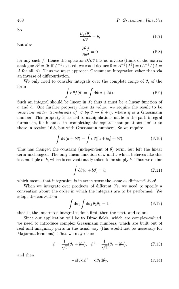
So
∂f (θ) = b,
(P.7)
∂θ
but also
∂
2 f = 0
(P.8)
∂θ 2
for any such f . Hence the operator ∂/∂θ has no inverse (think of the matrix
analogue A
2 = 0: if A
−1 existed, we could deduce 0 = A
−1 (A
2 ) = (A
−1 A)A =
A for all A). Thus we must approach Grassmann integration other than via
an inverse of differentiation.
We only need to consider integrals over the complete range of θ, of the
form
∫
∫
dθf (θ) = dθ(a + bθ).
(P.9)
Such an integral should be linear in f ; thus it must be a linear function of
a and b. One further property fixes its value: we require the result to be
invariant under translations of θ by θ → θ + η, where η is a Grassmann
number. This property is crucial to manipulations made in the path integral
formalism, for instance in ‘completing the square’ manipulations similar to
those in section 16.3, but with Grassmann numbers. So we require
∫
∫
dθ(a + bθ) = dθ([a + bη] + bθ).
(P.10)
This has changed the constant (independent of θ) term, but left the linear
term unchanged. The only linear function of a and b which behaves like this
is a multiple of b, which is conventionally taken to be simply b. Thus we define
∫
dθ(a + bθ) = b,
(P.11)
which means that integration is in some sense the same as differentiation!
When we integrate over products of different θ’s, we need to specify a
convention about the order in which the integrals are to be performed. We
adopt the convention
∫
∫
dθ 1 dθ 2 θ 2 θ 1 = 1 ;
(P.12)
that is, the innermost integral is done first, then the next, and so on.
Since our application will be to Dirac fields, which are complex-valued,
we need to introduce complex Grassmann numbers, which are built out of
real and imaginary parts in the usual way (this would not be necessary for
Majorana fermions). Thus we may define
1
1
ψ = √ (θ 1 + iθ 2 ), ψ
∗ = √ (θ 1 − iθ 2 ),
(P.13)
2
2
and then
−idψdψ
∗ = dθ 1 dθ 2 .
(P.14)
P. Grassmann Variables
So
∂f (θ) = b,
(P.7)
∂θ
but also
∂
2 f = 0
(P.8)
∂θ 2
for any such f . Hence the operator ∂/∂θ has no inverse (think of the matrix
analogue A
2 = 0: if A
−1 existed, we could deduce 0 = A
−1 (A
2 ) = (A
−1 A)A =
A for all A). Thus we must approach Grassmann integration other than via
an inverse of differentiation.
We only need to consider integrals over the complete range of θ, of the
form
∫
∫
dθf (θ) = dθ(a + bθ).
(P.9)
Such an integral should be linear in f ; thus it must be a linear function of
a and b. One further property fixes its value: we require the result to be
invariant under translations of θ by θ → θ + η, where η is a Grassmann
number. This property is crucial to manipulations made in the path integral
formalism, for instance in ‘completing the square’ manipulations similar to
those in section 16.3, but with Grassmann numbers. So we require
∫
∫
dθ(a + bθ) = dθ([a + bη] + bθ).
(P.10)
This has changed the constant (independent of θ) term, but left the linear
term unchanged. The only linear function of a and b which behaves like this
is a multiple of b, which is conventionally taken to be simply b. Thus we define
∫
dθ(a + bθ) = b,
(P.11)
which means that integration is in some sense the same as differentiation!
When we integrate over products of different θ’s, we need to specify a
convention about the order in which the integrals are to be performed. We
adopt the convention
∫
∫
dθ 1 dθ 2 θ 2 θ 1 = 1 ;
(P.12)
that is, the innermost integral is done first, then the next, and so on.
Since our application will be to Dirac fields, which are complex-valued,
we need to introduce complex Grassmann numbers, which are built out of
real and imaginary parts in the usual way (this would not be necessary for
Majorana fermions). Thus we may define
1
1
ψ = √ (θ 1 + iθ 2 ), ψ
∗ = √ (θ 1 − iθ 2 ),
(P.13)
2
2
and then
−idψdψ
∗ = dθ 1 dθ 2 .
(P.14)