

465
O. Dimensional Regularization
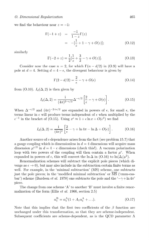
we find the behaviour near z = −1:
−1
Γ(−1 + z) = 1 − z
Γ(z)
1
= −[ + 1 − γ + O(z)];
(O.12)
z
similarly
1 1 3
Γ(−2 + z) = [ + − γ + O(z)].
(O.13)
2 z
2
Consider now the case n = 2, for which Γ(n − d/2) in (O.9) will have a
pole at d = 4. Setting d = 4 − ∈, the divergent behaviour is given by
2
Γ(2 − d/2) = − γ + O(∈)
(O.14)
∈
from (O.10). I d (Δ, 2) is then given by
[
]
i
2
Δ
−∈/2
I d (Δ, 2) =
− γ + O(∈) .
(O.15)
(4π) 2−∈/2
∈
When Δ
−∈/2 and (4π)
−2+∈/2 are expanded in powers of ∈, for small ∈, the
terms linear in ∈ will produce terms independent of ∈ when multiplied by the
∈
−1 in the bracket of (O.15). Using x
∈
≈ 1 + ∈ ln x + O(∈
2 ) we find
[
]
i
2
I d (Δ, 2) =
− γ + ln 4π − ln Δ + O(∈) .
(O.16)
(4π) 2 ∈
Another source of ∈-dependence arises from the fact (see problem 15.7) that
a gauge coupling which is dimensionless in d = 4 dimensions will acquire mass
dimension μ
∈/2 in d = 4 − ∈ dimensions (check this!). A vacuum polarization
loop with two powers of the coupling will then contain a factor μ
∈ . When
expanded in powers of ∈, this will convert the ln Δ in (O.16) to ln(Δ/μ
2 ).
Renormalization schemes will subtract the explicit pole pieces (which diverge as ∈ → 0), but may also include in the subtraction certain finite terms as
well. For example, in the ‘minimal subtraction’ (MS) scheme, one subtracts
just the pole pieces; in the ‘modified minimal subtraction’ or MS (‘emm-essbar’) scheme (Bardeen et al. 1978) one subtracts the pole and the ‘−γ + ln 4π’
piece.
The change from one scheme ‘A’ to another ‘B’ must involve a finite renormalization of the form (Ellis et al. 1966, section 2.5)
α
B = α
A (1 + A 1 α
A + . . .).
(O.17)
s
s
s
Note that this implies that the first two coefficients of the β function are
unchanged under this transformation, so that they are scheme-independent.
Subsequent coefficients are scheme-dependent, as is the QCD parameter Λ
O. Dimensional Regularization
we find the behaviour near z = −1:
−1
Γ(−1 + z) = 1 − z
Γ(z)
1
= −[ + 1 − γ + O(z)];
(O.12)
z
similarly
1 1 3
Γ(−2 + z) = [ + − γ + O(z)].
(O.13)
2 z
2
Consider now the case n = 2, for which Γ(n − d/2) in (O.9) will have a
pole at d = 4. Setting d = 4 − ∈, the divergent behaviour is given by
2
Γ(2 − d/2) = − γ + O(∈)
(O.14)
∈
from (O.10). I d (Δ, 2) is then given by
[
]
i
2
Δ
−∈/2
I d (Δ, 2) =
− γ + O(∈) .
(O.15)
(4π) 2−∈/2
∈
When Δ
−∈/2 and (4π)
−2+∈/2 are expanded in powers of ∈, for small ∈, the
terms linear in ∈ will produce terms independent of ∈ when multiplied by the
∈
−1 in the bracket of (O.15). Using x
∈
≈ 1 + ∈ ln x + O(∈
2 ) we find
[
]
i
2
I d (Δ, 2) =
− γ + ln 4π − ln Δ + O(∈) .
(O.16)
(4π) 2 ∈
Another source of ∈-dependence arises from the fact (see problem 15.7) that
a gauge coupling which is dimensionless in d = 4 dimensions will acquire mass
dimension μ
∈/2 in d = 4 − ∈ dimensions (check this!). A vacuum polarization
loop with two powers of the coupling will then contain a factor μ
∈ . When
expanded in powers of ∈, this will convert the ln Δ in (O.16) to ln(Δ/μ
2 ).
Renormalization schemes will subtract the explicit pole pieces (which diverge as ∈ → 0), but may also include in the subtraction certain finite terms as
well. For example, in the ‘minimal subtraction’ (MS) scheme, one subtracts
just the pole pieces; in the ‘modified minimal subtraction’ or MS (‘emm-essbar’) scheme (Bardeen et al. 1978) one subtracts the pole and the ‘−γ + ln 4π’
piece.
The change from one scheme ‘A’ to another ‘B’ must involve a finite renormalization of the form (Ellis et al. 1966, section 2.5)
α
B = α
A (1 + A 1 α
A + . . .).
(O.17)
s
s
s
Note that this implies that the first two coefficients of the β function are
unchanged under this transformation, so that they are scheme-independent.
Subsequent coefficients are scheme-dependent, as is the QCD parameter Λ