

466
O. Dimensional Regularization
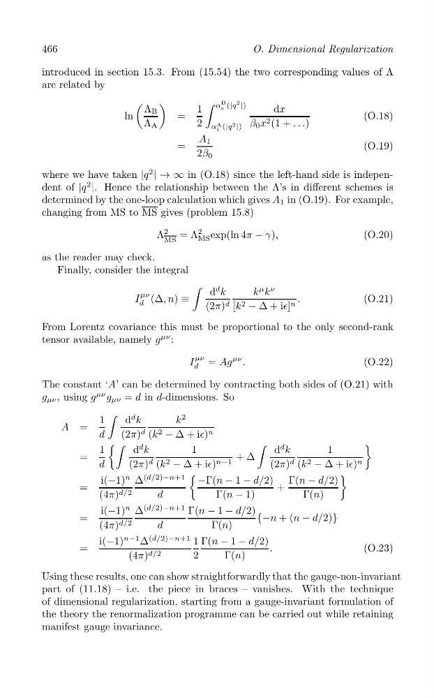
introduced in section 15.3. From (15.54) the two corresponding values of Λ
are related by
(
)
∫
Λ
1
α
B
2
s (
B
|q |)
dx
ln
=
(O.18)
Λ A
2 α A ( q 2 ) β 0 x 2 (1 + . . .)
s | |
A 1
=
(O.19)
2β 0
where we have taken |q
2
| → ∞ in (O.18) since the left-hand side is independent of |q
2
|. Hence the relationship between the Λ’s in different schemes is
determined by the one-loop calculation which gives A 1 in (O.19). For example,
changing from MS to MS gives (problem 15.8)
Λ
2
= Λ
2
MS exp(ln 4π − γ),
(O.20)
MS
as the reader may check.
Finally, consider the integral
∫ d
d k
k
μ k
ν
μν
I d (Δ, n) ≡
.
(O.21)
(2π) d [k 2 − Δ + i∈] n
From Lorentz covariance this must be proportional to the only second-rank
tensor available, namely g
μν :
μν
I = Ag
μν
d
.
(O.22)
The constant ‘A’ can be determined by contracting both sides of (O.21) with
g μν , using g
μν g μν = d in d-dimensions. So
∫
1
d
d k
k
2
A = d
(2π) d (k 2 − Δ + i∈) n
(∫
d
∫
d
)
1
d k
1
d k
1
=
+ Δ
d
(2π) d (k 2 − Δ + i∈) n−1
(2π) d (k 2 − Δ + i∈) n
)
i(−1)
n
n+1
(
Δ
(d/2)−
−Γ(n
Γ(
=
− 1
(4π) d/2
− d/2)
n
+
− d/2)
d
Γ(n − 1)
Γ(n)
i( 1)
n Δ
(d/2)−n+1 Γ(n 1 d/2)
=
−
− −
{−n + (n
(4π) d/2
d
Γ(n)
− d/2)}
i(−1)
n−1 Δ
(d/2)−n+1 1 Γ(n 1 d/
=
(4 ) d/2
− − 2) .
(O.23)
π
2
Γ(n)
Using these results, one can show straightforwardly that the gauge-non-invariant
part of (11.18) – i.e. the piece in braces – vanishes. With the technique
of dimensional regularization, starting from a gauge-invariant formulation of
the theory the renormalization programme can be carried out while retaining
manifest gauge invariance.
O. Dimensional Regularization
introduced in section 15.3. From (15.54) the two corresponding values of Λ
are related by
(
)
∫
Λ
1
α
B
2
s (
B
|q |)
dx
ln
=
(O.18)
Λ A
2 α A ( q 2 ) β 0 x 2 (1 + . . .)
s | |
A 1
=
(O.19)
2β 0
where we have taken |q
2
| → ∞ in (O.18) since the left-hand side is independent of |q
2
|. Hence the relationship between the Λ’s in different schemes is
determined by the one-loop calculation which gives A 1 in (O.19). For example,
changing from MS to MS gives (problem 15.8)
Λ
2
= Λ
2
MS exp(ln 4π − γ),
(O.20)
MS
as the reader may check.
Finally, consider the integral
∫ d
d k
k
μ k
ν
μν
I d (Δ, n) ≡
.
(O.21)
(2π) d [k 2 − Δ + i∈] n
From Lorentz covariance this must be proportional to the only second-rank
tensor available, namely g
μν :
μν
I = Ag
μν
d
.
(O.22)
The constant ‘A’ can be determined by contracting both sides of (O.21) with
g μν , using g
μν g μν = d in d-dimensions. So
∫
1
d
d k
k
2
A = d
(2π) d (k 2 − Δ + i∈) n
(∫
d
∫
d
)
1
d k
1
d k
1
=
+ Δ
d
(2π) d (k 2 − Δ + i∈) n−1
(2π) d (k 2 − Δ + i∈) n
)
i(−1)
n
n+1
(
Δ
(d/2)−
−Γ(n
Γ(
=
− 1
(4π) d/2
− d/2)
n
+
− d/2)
d
Γ(n − 1)
Γ(n)
i( 1)
n Δ
(d/2)−n+1 Γ(n 1 d/2)
=
−
− −
{−n + (n
(4π) d/2
d
Γ(n)
− d/2)}
i(−1)
n−1 Δ
(d/2)−n+1 1 Γ(n 1 d/
=
(4 ) d/2
− − 2) .
(O.23)
π
2
Γ(n)
Using these results, one can show straightforwardly that the gauge-non-invariant
part of (11.18) – i.e. the piece in braces – vanishes. With the technique
of dimensional regularization, starting from a gauge-invariant formulation of
the theory the renormalization programme can be carried out while retaining
manifest gauge invariance.