

O
Dimensional Regularization
After combining propagator denominators of the form (p
2
− m
2 + i∈)
−1 by
Feynman parameters (cf (10.40)), and shifting the origin of the loop momentum to complete the square (cf (10.42) and (11.16)), all one-loop Feynman
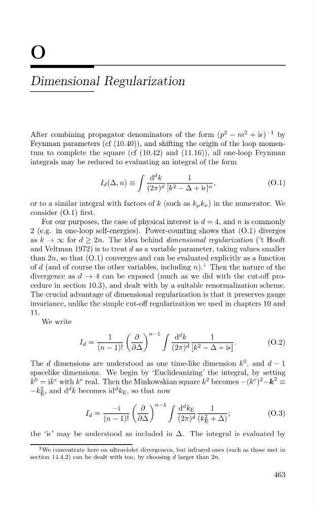
integrals may be reduced to evaluating an integral of the form
∫ d
d k
1
I d (Δ, n) ≡
,
(O.1)
(2π) d [k 2 − Δ + i∈] n
or to a similar integral with factors of k (such as k μ k ν ) in the numerator. We
consider (O.1) first.
For our purposes, the case of physical interest is d = 4, and n is commonly
2 (e.g. in one-loop self-energies). Power-counting shows that (O.1) diverges
as k → ∞ for d ≥ 2n. The idea behind dimensional regularization (’t Hooft
and Veltman 1972) is to treat d as a variable parameter, taking values smaller
than 2n, so that (O.1) converges and can be evaluated explicitly as a function
of d (and of course the other variables, including n).
1 Then the nature of the
divergence as d → 4 can be exposed (much as we did with the cut-off procedure in section 10.3), and dealt with by a suitable renormalization scheme.
The crucial advantage of dimensional regularization is that it preserves gauge
invariance, unlike the simple cut-off regularization we used in chapters 10 and
11.
We write
(
) n 1 ∫
1
∂
−
d
d k
1
I d =
.
(O.2)
(n − 1)! ∂Δ
(2π) d [k 2 − Δ + i∈]
The d dimensions are understood as one time-like dimension k
0 , and d − 1
spacelike dimensions. We begin by ‘Euclideanizing’ the integral, by setting
k
0 = ik
e with k
e real. Then the Minkowskian square k
2 becomes −(k
e )
2
−k
2
2
≡
−k E , and d
d k becomes id
d k E , so that now
(
)
−
n 1 ∫
i
∂
−
d
d k E
1
I d =
;
(O.3)
(n − 1)! ∂Δ
(2π) d (k 2
E + Δ)
the ‘i∈’ may be understood as included in Δ. The integral is evaluated by
1 We concentrate here on ultraviolet divergences, but infrared ones (such as those met in
section 14.4.2) can be dealt with too, by choosing d larger than 2n.
463
Dimensional Regularization
After combining propagator denominators of the form (p
2
− m
2 + i∈)
−1 by
Feynman parameters (cf (10.40)), and shifting the origin of the loop momentum to complete the square (cf (10.42) and (11.16)), all one-loop Feynman
integrals may be reduced to evaluating an integral of the form
∫ d
d k
1
I d (Δ, n) ≡
,
(O.1)
(2π) d [k 2 − Δ + i∈] n
or to a similar integral with factors of k (such as k μ k ν ) in the numerator. We
consider (O.1) first.
For our purposes, the case of physical interest is d = 4, and n is commonly
2 (e.g. in one-loop self-energies). Power-counting shows that (O.1) diverges
as k → ∞ for d ≥ 2n. The idea behind dimensional regularization (’t Hooft
and Veltman 1972) is to treat d as a variable parameter, taking values smaller
than 2n, so that (O.1) converges and can be evaluated explicitly as a function
of d (and of course the other variables, including n).
1 Then the nature of the
divergence as d → 4 can be exposed (much as we did with the cut-off procedure in section 10.3), and dealt with by a suitable renormalization scheme.
The crucial advantage of dimensional regularization is that it preserves gauge
invariance, unlike the simple cut-off regularization we used in chapters 10 and
11.
We write
(
) n 1 ∫
1
∂
−
d
d k
1
I d =
.
(O.2)
(n − 1)! ∂Δ
(2π) d [k 2 − Δ + i∈]
The d dimensions are understood as one time-like dimension k
0 , and d − 1
spacelike dimensions. We begin by ‘Euclideanizing’ the integral, by setting
k
0 = ik
e with k
e real. Then the Minkowskian square k
2 becomes −(k
e )
2
−k
2
2
≡
−k E , and d
d k becomes id
d k E , so that now
(
)
−
n 1 ∫
i
∂
−
d
d k E
1
I d =
;
(O.3)
(n − 1)! ∂Δ
(2π) d (k 2
E + Δ)
the ‘i∈’ may be understood as included in Δ. The integral is evaluated by
1 We concentrate here on ultraviolet divergences, but infrared ones (such as those met in
section 14.4.2) can be dealt with too, by choosing d larger than 2n.
463