

462
N. Geometrical Aspects of Gauge Fields
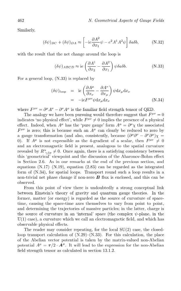
Similarly,
[
]
∂A
2
(δψ) BC + (δψ) DA ≈ −ie
ψ − e
2 A
1 A
2 ψ δaδb,
(N.32)
∂x 1
with the result that the net change around the loop is
(
)
∂A
1
∂A
2
(δψ) ABCD ≈ ie
−
ψδaδb.
(N.33)
∂x 2
∂x 1
For a general loop, (N.33) is replaced by
(
)
∂A
μ
∂A
ν
(δψ) loop = ie
−
ψdx μ dx ν
∂x ν
∂x μ
= −ieF
μν ψdx μ dx ν
(N.34)
where F
μν = ∂
μ A
ν
− ∂
ν A
μ is the familiar field strength tensor of QED.
The analogy we have been pursuing would therefore suggest that F
μν = 0
indicates ‘no physical effect’, while F
μν
/ 0 implies the presence of a physical
=
effect. Indeed, when A
μ has the ‘pure gauge’ form A
μ = ∂
μ χ the associated
F
μν is zero; this is because such an A
μ can clearly be reduced to zero by
a gauge transformation (and also, consistently, because (∂
μ ∂
ν
− ∂
ν ∂
μ )χ =
0). If A
μ
/
is not expressible as the 4-gradient of a scalar, then F
μν = 0
and an electromagnetic field is present, analogous to the spatial curvature
revealed by R
α
/ 0. Once again, there is a satisfying consistency between
=
γβσ
this ‘geometrical’ viewpoint and the discussion of the Aharonov-Bohm effect
in Section 2.6. As in our remarks at the end of the previous section, and
equations (N.17)–(N.19), equation (2.83) can be regarded as the integrated
form of (N.34), for spatial loops. Transport round such a loop results in a
non-trivial net phase change if non-zero B flux is enclosed, and this can be
observed.
From this point of view there is undoubtedly a strong conceptual link
between Einstein’s theory of gravity and quantum gauge theories. In the
former, matter (or energy) is regarded as the source of curvature of spacetime, causing the space-time axes themselves to vary from point to point,
and determining the trajectories of massive particles; in the latter, charge is
the source of curvature in an ‘internal’ space (the complex ψ-plane, in the
U(1) case), a curvature which we call an electromagnetic field, and which has
observable physical effects.
The reader may consider repeating, for the local SU(2) case, the closedloop transport calculation of (N.29)–(N.33). For this calculation, the place
of the Abelian vector potential is taken by the matrix-valued non-Abelian
potential A
μ = τ /2 · A
μ . It will lead to the expression for the non-Abelian
field strength tensor as calculated in section 13.1.2.
N. Geometrical Aspects of Gauge Fields
Similarly,
[
]
∂A
2
(δψ) BC + (δψ) DA ≈ −ie
ψ − e
2 A
1 A
2 ψ δaδb,
(N.32)
∂x 1
with the result that the net change around the loop is
(
)
∂A
1
∂A
2
(δψ) ABCD ≈ ie
−
ψδaδb.
(N.33)
∂x 2
∂x 1
For a general loop, (N.33) is replaced by
(
)
∂A
μ
∂A
ν
(δψ) loop = ie
−
ψdx μ dx ν
∂x ν
∂x μ
= −ieF
μν ψdx μ dx ν
(N.34)
where F
μν = ∂
μ A
ν
− ∂
ν A
μ is the familiar field strength tensor of QED.
The analogy we have been pursuing would therefore suggest that F
μν = 0
indicates ‘no physical effect’, while F
μν
/ 0 implies the presence of a physical
=
effect. Indeed, when A
μ has the ‘pure gauge’ form A
μ = ∂
μ χ the associated
F
μν is zero; this is because such an A
μ can clearly be reduced to zero by
a gauge transformation (and also, consistently, because (∂
μ ∂
ν
− ∂
ν ∂
μ )χ =
0). If A
μ
/
is not expressible as the 4-gradient of a scalar, then F
μν = 0
and an electromagnetic field is present, analogous to the spatial curvature
revealed by R
α
/ 0. Once again, there is a satisfying consistency between
=
γβσ
this ‘geometrical’ viewpoint and the discussion of the Aharonov-Bohm effect
in Section 2.6. As in our remarks at the end of the previous section, and
equations (N.17)–(N.19), equation (2.83) can be regarded as the integrated
form of (N.34), for spatial loops. Transport round such a loop results in a
non-trivial net phase change if non-zero B flux is enclosed, and this can be
observed.
From this point of view there is undoubtedly a strong conceptual link
between Einstein’s theory of gravity and quantum gauge theories. In the
former, matter (or energy) is regarded as the source of curvature of spacetime, causing the space-time axes themselves to vary from point to point,
and determining the trajectories of massive particles; in the latter, charge is
the source of curvature in an ‘internal’ space (the complex ψ-plane, in the
U(1) case), a curvature which we call an electromagnetic field, and which has
observable physical effects.
The reader may consider repeating, for the local SU(2) case, the closedloop transport calculation of (N.29)–(N.33). For this calculation, the place
of the Abelian vector potential is taken by the matrix-valued non-Abelian
potential A
μ = τ /2 · A
μ . It will lead to the expression for the non-Abelian
field strength tensor as calculated in section 13.1.2.