

461
N.2. Geometrical curvature and the gauge field strength tensor
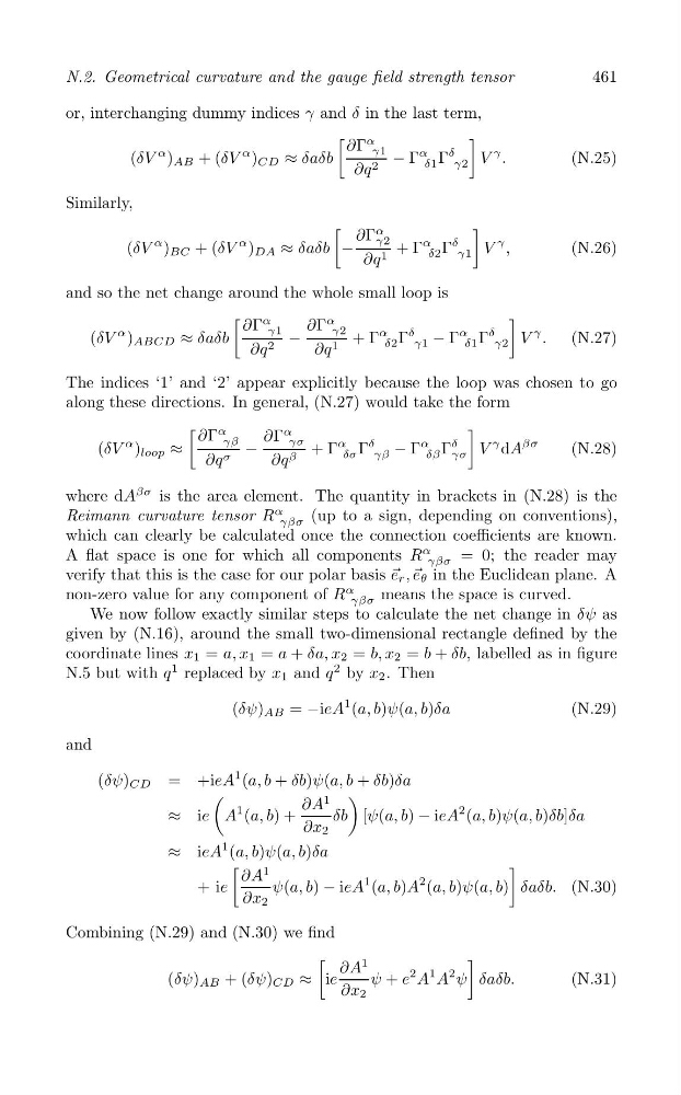
or, interchanging dummy indices γ and δ in the last term,
[
]
∂Γ
α
γ1
(δV
α ) AB + (δV
α ) CD ≈ δaδb
− Γ
α
δ1 Γ
δ
γ2 V
γ .
(N.25)
∂q 2
Similarly,
[
]
∂Γ
α
γ2
(δV
α ) BC + (δV
α ) DA ≈ δaδb −
+ Γ
α
δ2 Γ
δ
V
γ ,
(N.26)
γ1
∂q 1
and so the net change around the whole small loop is
[
]
∂Γ
α
∂Γ
α
γ1
γ2
(δV
α ) ABCD ≈ δaδb
−
+ Γ
α
δ2 Γ
δ
γ1 − Γ
α
δ1 Γ
δ
V
γ . (N.27)
γ2
∂q 2
∂q 1
The indices ‘1’ and ‘2’ appear explicitly because the loop was chosen to go
along these directions. In general, (N.27) would take the form
[
]
∂Γ
α
γβ
∂Γ
α
γσ
V
γ dA
βσ
(δV
α ) loop ≈
−
+ Γ
α
δσ Γ
δ
γβ − Γ
α
δβ Γ
δ
(N.28)
γσ
∂q σ
∂q β
where dA
βσ is the area element. The quantity in brackets in (N.28) is the
Reimann curvature tensor R
α
γβσ (up to a sign, depending on conventions),
which can clearly be calculated once the connection coefficients are known.
A flat space is one for which all components R
α
= 0; the reader may
γβσ
verify that this is the case for our polar basis → e r , → e θ in the Euclidean plane. A
non-zero value for any component of R
α
means the space is curved.
γβσ
We now follow exactly similar steps to calculate the net change in δψ as
given by (N.16), around the small two-dimensional rectangle defined by the
coordinate lines x 1 = a, x 1 = a + δa, x 2 = b, x 2 = b + δb, labelled as in figure
N.5 but with q
1 replaced by x 1 and q
2 by x 2 . Then
(δψ) AB = −ieA
1 (a, b)ψ(a, b)δa
(N.29)
and
(δψ) CD = +ieA
1 (a, b + δb)ψ(a, b + δb)δa
(
)
∂A
1
≈ ie A
1 (a, b) +
δb [ψ(a, b) − ieA
2 (a, b)ψ(a, b)δb]δa
∂x 2
≈ ieA
1 (a, b)ψ(a, b)δa
[
]
∂A
1
+ ie
ψ(a, b) − ieA
1 (a, b)A
2 (a, b)ψ(a, b) δaδb. (N.30)
∂x 2
Combining (N.29) and (N.30) we find
[
]
∂A
1
2 A
1 A
2 ψ
(δψ) AB + (δψ) CD ≈ ie
ψ + e
δaδb.
(N.31)
∂x 2
N.2. Geometrical curvature and the gauge field strength tensor
or, interchanging dummy indices γ and δ in the last term,
[
]
∂Γ
α
γ1
(δV
α ) AB + (δV
α ) CD ≈ δaδb
− Γ
α
δ1 Γ
δ
γ2 V
γ .
(N.25)
∂q 2
Similarly,
[
]
∂Γ
α
γ2
(δV
α ) BC + (δV
α ) DA ≈ δaδb −
+ Γ
α
δ2 Γ
δ
V
γ ,
(N.26)
γ1
∂q 1
and so the net change around the whole small loop is
[
]
∂Γ
α
∂Γ
α
γ1
γ2
(δV
α ) ABCD ≈ δaδb
−
+ Γ
α
δ2 Γ
δ
γ1 − Γ
α
δ1 Γ
δ
V
γ . (N.27)
γ2
∂q 2
∂q 1
The indices ‘1’ and ‘2’ appear explicitly because the loop was chosen to go
along these directions. In general, (N.27) would take the form
[
]
∂Γ
α
γβ
∂Γ
α
γσ
V
γ dA
βσ
(δV
α ) loop ≈
−
+ Γ
α
δσ Γ
δ
γβ − Γ
α
δβ Γ
δ
(N.28)
γσ
∂q σ
∂q β
where dA
βσ is the area element. The quantity in brackets in (N.28) is the
Reimann curvature tensor R
α
γβσ (up to a sign, depending on conventions),
which can clearly be calculated once the connection coefficients are known.
A flat space is one for which all components R
α
= 0; the reader may
γβσ
verify that this is the case for our polar basis → e r , → e θ in the Euclidean plane. A
non-zero value for any component of R
α
means the space is curved.
γβσ
We now follow exactly similar steps to calculate the net change in δψ as
given by (N.16), around the small two-dimensional rectangle defined by the
coordinate lines x 1 = a, x 1 = a + δa, x 2 = b, x 2 = b + δb, labelled as in figure
N.5 but with q
1 replaced by x 1 and q
2 by x 2 . Then
(δψ) AB = −ieA
1 (a, b)ψ(a, b)δa
(N.29)
and
(δψ) CD = +ieA
1 (a, b + δb)ψ(a, b + δb)δa
(
)
∂A
1
≈ ie A
1 (a, b) +
δb [ψ(a, b) − ieA
2 (a, b)ψ(a, b)δb]δa
∂x 2
≈ ieA
1 (a, b)ψ(a, b)δa
[
]
∂A
1
+ ie
ψ(a, b) − ieA
1 (a, b)A
2 (a, b)ψ(a, b) δaδb. (N.30)
∂x 2
Combining (N.29) and (N.30) we find
[
]
∂A
1
2 A
1 A
2 ψ
(δψ) AB + (δψ) CD ≈ ie
ψ + e
δaδb.
(N.31)
∂x 2