

458
N. Geometrical Aspects of Gauge Fields
has been carried by ‘parallel transport’ from one point to the other; they are
often called ‘connection coefficients’, or just ‘the connection’.
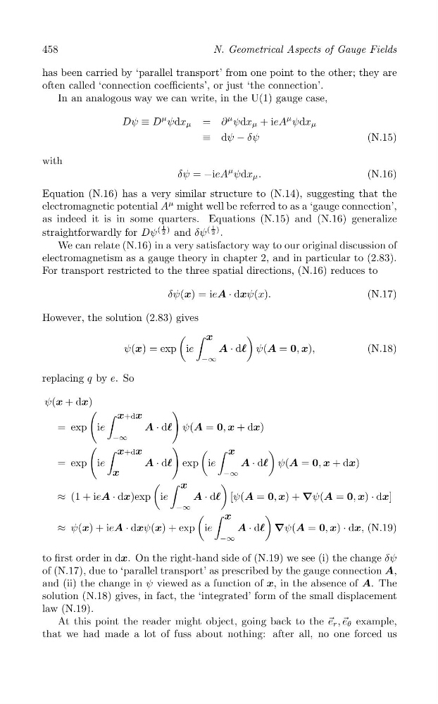
In an analogous way we can write, in the U(1) gauge case,
Dψ ≡ D
μ ψdx μ = ∂
μ ψdx μ + ieA
μ ψdx μ
≡ dψ − δψ
(N.15)
with
δψ = −ieA
μ ψdx μ .
(N.16)
Equation (N.16) has a very similar structure to (N.14), suggesting that the
electromagnetic potential A
μ might well be referred to as a ‘gauge connection’,
as indeed it is in some quarters. Equations (N.15) and (N.16) generalize
straightforwardly for Dψ
(
1
2 ) and δψ
(
1
2 ) .
We can relate (N.16) in a very satisfactory way to our original discussion of
electromagnetism as a gauge theory in chapter 2, and in particular to (2.83).
For transport restricted to the three spatial directions, (N.16) reduces to
δψ(x) = ieA · dxψ(x).
(N.17)
However, the solution (2.83) gives
( ∫
)
x
ψ(x) = exp ie
A · de ψ(A = 0, x),
(N.18)
−∞
replacing q by e. So
ψ(x + dx)
(
)
∫ x+dx
= exp ie
A · de ψ(A = 0, x + dx)
−∞
( ∫
)
( ∫
)
x+dx
x
= exp ie
A · de exp ie
A · de ψ(A = 0, x + dx)
x
−∞
( ∫
)
x
≈ (1 + ieA · dx)exp ie
A · de [ψ(A = 0, x) + ∇ψ(A = 0, x) · dx]
−∞ ( ∫
)
x
≈ ψ(x) + ieA · dxψ(x) + exp ie
A · de ∇ψ(A = 0, x) · dx, (N.19)
−∞
to first order in dx. On the right-hand side of (N.19) we see (i) the change δψ
of (N.17), due to ‘parallel transport’ as prescribed by the gauge connection A,
and (ii) the change in ψ viewed as a function of x, in the absence of A. The
solution (N.18) gives, in fact, the ‘integrated’ form of the small displacement
law (N.19).
At this point the reader might object, going back to the → e r , → e θ example,
that we had made a lot of fuss about nothing: after all, no one forced us
N. Geometrical Aspects of Gauge Fields
has been carried by ‘parallel transport’ from one point to the other; they are
often called ‘connection coefficients’, or just ‘the connection’.
In an analogous way we can write, in the U(1) gauge case,
Dψ ≡ D
μ ψdx μ = ∂
μ ψdx μ + ieA
μ ψdx μ
≡ dψ − δψ
(N.15)
with
δψ = −ieA
μ ψdx μ .
(N.16)
Equation (N.16) has a very similar structure to (N.14), suggesting that the
electromagnetic potential A
μ might well be referred to as a ‘gauge connection’,
as indeed it is in some quarters. Equations (N.15) and (N.16) generalize
straightforwardly for Dψ
(
1
2 ) and δψ
(
1
2 ) .
We can relate (N.16) in a very satisfactory way to our original discussion of
electromagnetism as a gauge theory in chapter 2, and in particular to (2.83).
For transport restricted to the three spatial directions, (N.16) reduces to
δψ(x) = ieA · dxψ(x).
(N.17)
However, the solution (2.83) gives
( ∫
)
x
ψ(x) = exp ie
A · de ψ(A = 0, x),
(N.18)
−∞
replacing q by e. So
ψ(x + dx)
(
)
∫ x+dx
= exp ie
A · de ψ(A = 0, x + dx)
−∞
( ∫
)
( ∫
)
x+dx
x
= exp ie
A · de exp ie
A · de ψ(A = 0, x + dx)
x
−∞
( ∫
)
x
≈ (1 + ieA · dx)exp ie
A · de [ψ(A = 0, x) + ∇ψ(A = 0, x) · dx]
−∞ ( ∫
)
x
≈ ψ(x) + ieA · dxψ(x) + exp ie
A · de ∇ψ(A = 0, x) · dx, (N.19)
−∞
to first order in dx. On the right-hand side of (N.19) we see (i) the change δψ
of (N.17), due to ‘parallel transport’ as prescribed by the gauge connection A,
and (ii) the change in ψ viewed as a function of x, in the absence of A. The
solution (N.18) gives, in fact, the ‘integrated’ form of the small displacement
law (N.19).
At this point the reader might object, going back to the → e r , → e θ example,
that we had made a lot of fuss about nothing: after all, no one forced us