

459
N.1. Covariant derivatives and coordinate transformations
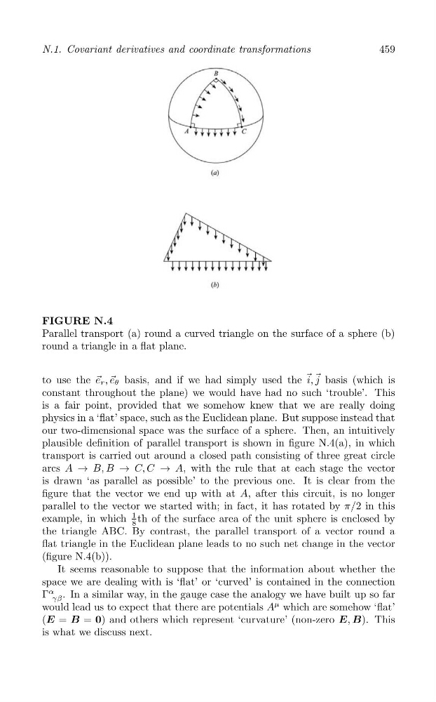
FIGURE N.4
Parallel transport (a) round a curved triangle on the surface of a sphere (b)
round a triangle in a flat plane.
to use the → e r , → e θ basis, and if we had simply used the → i, → j basis (which is
constant throughout the plane) we would have had no such ‘trouble’. This
is a fair point, provided that we somehow knew that we are really doing
physics in a ‘flat’ space, such as the Euclidean plane. But suppose instead that
our two-dimensional space was the surface of a sphere. Then, an intuitively
plausible definition of parallel transport is shown in figure N.4(a), in which
transport is carried out around a closed path consisting of three great circle
arcs A → B, B → C, C → A, with the rule that at each stage the vector
is drawn ‘as parallel as possible’ to the previous one. It is clear from the
figure that the vector we end up with at A, after this circuit, is no longer
parallel to the vector we started with; in fact, it has rotated by π/2 in this
example, in which
1 th of the surface area of the unit sphere is enclosed by
8
the triangle ABC. By contrast, the parallel transport of a vector round a
flat triangle in the Euclidean plane leads to no such net change in the vector
(figure N.4(b)).
It seems reasonable to suppose that the information about whether the
space we are dealing with is ‘flat’ or ‘curved’ is contained in the connection
Γ
α . In a similar way, in the gauge case the analogy we have built up so far
γβ
would lead us to expect that there are potentials A
μ which are somehow ‘flat’
(E = B = 0) and others which represent ‘curvature’ (non-zero E, B). This
is what we discuss next.
N.1. Covariant derivatives and coordinate transformations
FIGURE N.4
Parallel transport (a) round a curved triangle on the surface of a sphere (b)
round a triangle in a flat plane.
to use the → e r , → e θ basis, and if we had simply used the → i, → j basis (which is
constant throughout the plane) we would have had no such ‘trouble’. This
is a fair point, provided that we somehow knew that we are really doing
physics in a ‘flat’ space, such as the Euclidean plane. But suppose instead that
our two-dimensional space was the surface of a sphere. Then, an intuitively
plausible definition of parallel transport is shown in figure N.4(a), in which
transport is carried out around a closed path consisting of three great circle
arcs A → B, B → C, C → A, with the rule that at each stage the vector
is drawn ‘as parallel as possible’ to the previous one. It is clear from the
figure that the vector we end up with at A, after this circuit, is no longer
parallel to the vector we started with; in fact, it has rotated by π/2 in this
example, in which
1 th of the surface area of the unit sphere is enclosed by
8
the triangle ABC. By contrast, the parallel transport of a vector round a
flat triangle in the Euclidean plane leads to no such net change in the vector
(figure N.4(b)).
It seems reasonable to suppose that the information about whether the
space we are dealing with is ‘flat’ or ‘curved’ is contained in the connection
Γ
α . In a similar way, in the gauge case the analogy we have built up so far
γβ
would lead us to expect that there are potentials A
μ which are somehow ‘flat’
(E = B = 0) and others which represent ‘curvature’ (non-zero E, B). This
is what we discuss next.