

457
N.1. Covariant derivatives and coordinate transformations
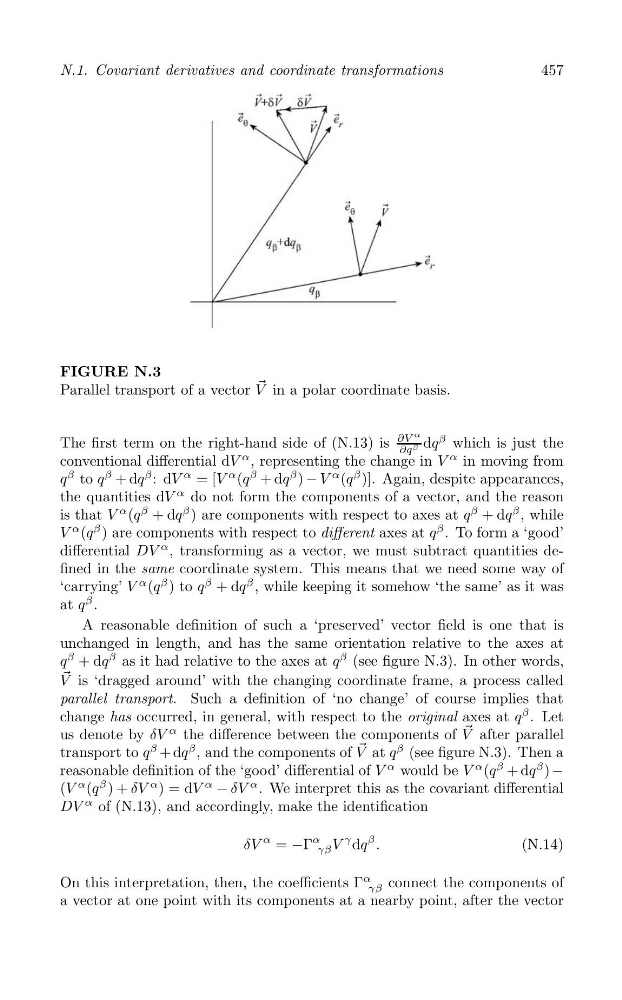
FIGURE N.3
Parallel transport of a vector V → in a polar coordinate basis.
β
The first term on the right-hand side of (N.13) is
∂V
α
dq which is just the
∂q β
conventional differential dV
α , representing the change in V
α in moving from
β
q to q
β + dq
β : dV
α = [V
α (q
β + dq
β ) − V
α (q
β )]. Again, despite appearances,
the quantities dV
α do not form the components of a vector, and the reason
is that V
α (q
β + dq
β ) are components with respect to axes at q
β + dq
β , while
V
α (q
β ) are components with respect to different axes at q
β . To form a ‘good’
differential DV
α , transforming as a vector, we must subtract quantities defined in the same coordinate system. This means that we need some way of
‘carrying’ V
α (q
β ) to q
β + dq
β , while keeping it somehow ‘the same’ as it was
at q
β .
A reasonable definition of such a ‘preserved’ vector field is one that is
unchanged in length, and has the same orientation relative to the axes at
q
β + dq
β as it had relative to the axes at q
β (see figure N.3). In other words,
→
V is ‘dragged around’ with the changing coordinate frame, a process called
parallel transport. Such a definition of ‘no change’ of course implies that
change has occurred, in general, with respect to the original axes at q
β . Let
us denote by δV
α the difference between the components of V → after parallel
β
transport to q
β + dq , and the components of V → at q
β (see figure N.3). Then a
reasonable definition of the ‘good’ differential of V
α would be V
α (q
β + dq
β ) −
(V
α (q
β ) + δV
α ) = dV
α
− δV
α . We interpret this as the covariant differential
DV
α of (N.13), and accordingly, make the identification
β
δV
α = −Γ
α
γβ V
γ dq .
(N.14)
On this interpretation, then, the coefficients Γ
α
connect the components of
γβ
a vector at one point with its components at a nearby point, after the vector
N.1. Covariant derivatives and coordinate transformations
FIGURE N.3
Parallel transport of a vector V → in a polar coordinate basis.
β
The first term on the right-hand side of (N.13) is
∂V
α
dq which is just the
∂q β
conventional differential dV
α , representing the change in V
α in moving from
β
q to q
β + dq
β : dV
α = [V
α (q
β + dq
β ) − V
α (q
β )]. Again, despite appearances,
the quantities dV
α do not form the components of a vector, and the reason
is that V
α (q
β + dq
β ) are components with respect to axes at q
β + dq
β , while
V
α (q
β ) are components with respect to different axes at q
β . To form a ‘good’
differential DV
α , transforming as a vector, we must subtract quantities defined in the same coordinate system. This means that we need some way of
‘carrying’ V
α (q
β ) to q
β + dq
β , while keeping it somehow ‘the same’ as it was
at q
β .
A reasonable definition of such a ‘preserved’ vector field is one that is
unchanged in length, and has the same orientation relative to the axes at
q
β + dq
β as it had relative to the axes at q
β (see figure N.3). In other words,
→
V is ‘dragged around’ with the changing coordinate frame, a process called
parallel transport. Such a definition of ‘no change’ of course implies that
change has occurred, in general, with respect to the original axes at q
β . Let
us denote by δV
α the difference between the components of V → after parallel
β
transport to q
β + dq , and the components of V → at q
β (see figure N.3). Then a
reasonable definition of the ‘good’ differential of V
α would be V
α (q
β + dq
β ) −
(V
α (q
β ) + δV
α ) = dV
α
− δV
α . We interpret this as the covariant differential
DV
α of (N.13), and accordingly, make the identification
β
δV
α = −Γ
α
γβ V
γ dq .
(N.14)
On this interpretation, then, the coefficients Γ
α
connect the components of
γβ
a vector at one point with its components at a nearby point, after the vector