

448
M. Group Theory
(the limit of every convergent sequence of points in the set also lies in the set).
For the Lorentz group, the limiting velocity c is not included (the γ-factor goes
to infinity), and so the group is non-compact.
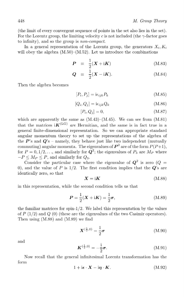
In a general representation of the Lorentz group, the generators X i , K i
will obey the algebra (M.50)–(M.52). Let us introduce the combinations
1 (X + iK)
(M.83)
P ≡ 2
1
Q ≡
(X − iK).
(M.84)
2
Then the algebra becomes
[P i , P j ] = i∈ ijk P k
(M.85)
[Q i , Q j ] = i∈ ijk Q k
(M.86)
[P i , Q j ] = 0,
(M.87)
which are apparently the same as (M.43)–(M.45). We can see from (M.81)
that the matrices iK
(LG) are Hermitian, and the same is in fact true in a
general finite-dimensional representation. So we can appropriate standard
angular momentum theory to set up the representations of the algebra of
the P ’s and Q’s – namely, they behave just like two independent (mutually
commuting) angular momenta. The eigenvalues of P
2 are of the form P (P +1),
for P = 0, 1/2, . . ., and similarly for Q
2 ; the eigenvalues of P 3 are M P where
−P ≤ M P ≤ P , and similarly for Q 3 .
Consider the particular case where the eigenvalue of Q
2 is zero (Q =
0), and the value of P is 1/2. The first condition implies that the Q’s are
identically zero, so that
X = iK
(M.88)
in this representation, while the second condition tells us that
1
1
P = (X + iK) = σ,
(M.89)
2
2
the familiar matrices for spin-1/2. We label this representation by the values
of P (1/2) and Q (0) (these are the eigenvalues of the two Casimir operators).
Then using (M.88) and (M.89) we find
,0)
1
= σ
(M.90)
2
1
2
X
(
and
i
1
2
K
( ,0) = − σ.
(M.91)
2
Now recall that the general infinitesimal Lorentz transformation has the
form
1 + i∊ · X − iη · K.
(M.92)
M. Group Theory
(the limit of every convergent sequence of points in the set also lies in the set).
For the Lorentz group, the limiting velocity c is not included (the γ-factor goes
to infinity), and so the group is non-compact.
In a general representation of the Lorentz group, the generators X i , K i
will obey the algebra (M.50)–(M.52). Let us introduce the combinations
1 (X + iK)
(M.83)
P ≡ 2
1
Q ≡
(X − iK).
(M.84)
2
Then the algebra becomes
[P i , P j ] = i∈ ijk P k
(M.85)
[Q i , Q j ] = i∈ ijk Q k
(M.86)
[P i , Q j ] = 0,
(M.87)
which are apparently the same as (M.43)–(M.45). We can see from (M.81)
that the matrices iK
(LG) are Hermitian, and the same is in fact true in a
general finite-dimensional representation. So we can appropriate standard
angular momentum theory to set up the representations of the algebra of
the P ’s and Q’s – namely, they behave just like two independent (mutually
commuting) angular momenta. The eigenvalues of P
2 are of the form P (P +1),
for P = 0, 1/2, . . ., and similarly for Q
2 ; the eigenvalues of P 3 are M P where
−P ≤ M P ≤ P , and similarly for Q 3 .
Consider the particular case where the eigenvalue of Q
2 is zero (Q =
0), and the value of P is 1/2. The first condition implies that the Q’s are
identically zero, so that
X = iK
(M.88)
in this representation, while the second condition tells us that
1
1
P = (X + iK) = σ,
(M.89)
2
2
the familiar matrices for spin-1/2. We label this representation by the values
of P (1/2) and Q (0) (these are the eigenvalues of the two Casimir operators).
Then using (M.88) and (M.89) we find
,0)
1
= σ
(M.90)
2
1
2
X
(
and
i
1
2
K
( ,0) = − σ.
(M.91)
2
Now recall that the general infinitesimal Lorentz transformation has the
form
1 + i∊ · X − iη · K.
(M.92)