

391
22.3. Simple (tree-level) predictions
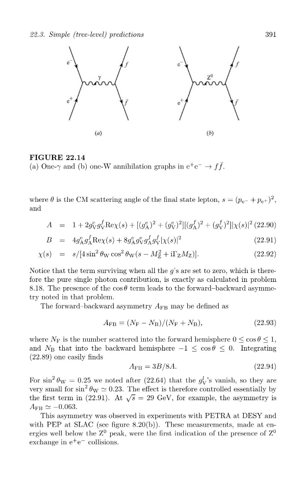
FIGURE 22.14
¯
(a) One-γ and (b) one-W annihilation graphs in e
+ e
−
→ f f .
where θ is the CM scattering angle of the final state lepton, s = (p e − + p e + )
2 ,
and
e f
V g V
f
A )
2 + (g
f
V
e
e
A )
2 + (g V )
2 ][(g
)
2 ]|χ(s)|
2 (22.90)
A = 1 + 2g
Reχ(s) + [(g
f
f
f
2
e
e e
|χ(s)|
Reχ(s) + 8g
(22.91)
B = 4g A g
A g V g A g
A
V
χ(s) = s/[4 sin
2 θ W cos
2 θ W (s − M Z
2 + iΓ Z M Z )].
(22.92)
Notice that the term surviving when all the g’s are set to zero, which is therefore the pure single photon contribution, is exactly as calculated in problem
8.18. The presence of the cos θ term leads to the forward–backward asymmetry noted in that problem.
The forward–backward asymmetry A FB may be defined as
A FB ≡ (N F − N B )/(N F + N B ),
(22.93)
where N F is the number scattered into the forward hemisphere 0 ≤ cos θ ≤ 1,
and N B that into the backward hemisphere −1 ≤ cos θ ≤ 0. Integrating
(22.89) one easily finds
A FB = 3B/8A.
(22.94)
For sin
2 θ W = 0.25 we noted after (22.64) that the g
l
V ’s vanish, so they are
very small for sin
2 θ W ⋍ 0.23. The effect is therefore controlled essentially by
√
the first term in (22.91). At s = 29 GeV, for example, the asymmetry is
A FB ⋍ −0.063.
This asymmetry was observed in experiments with PETRA at DESY and
with PEP at SLAC (see figure 8.20(b)). These measurements, made at energies well below the Z
0 peak, were the first indication of the presence of Z
0
exchange in e
+ e
− collisions.
22.3. Simple (tree-level) predictions
FIGURE 22.14
¯
(a) One-γ and (b) one-W annihilation graphs in e
+ e
−
→ f f .
where θ is the CM scattering angle of the final state lepton, s = (p e − + p e + )
2 ,
and
e f
V g V
f
A )
2 + (g
f
V
e
e
A )
2 + (g V )
2 ][(g
)
2 ]|χ(s)|
2 (22.90)
A = 1 + 2g
Reχ(s) + [(g
f
f
f
2
e
e e
|χ(s)|
Reχ(s) + 8g
(22.91)
B = 4g A g
A g V g A g
A
V
χ(s) = s/[4 sin
2 θ W cos
2 θ W (s − M Z
2 + iΓ Z M Z )].
(22.92)
Notice that the term surviving when all the g’s are set to zero, which is therefore the pure single photon contribution, is exactly as calculated in problem
8.18. The presence of the cos θ term leads to the forward–backward asymmetry noted in that problem.
The forward–backward asymmetry A FB may be defined as
A FB ≡ (N F − N B )/(N F + N B ),
(22.93)
where N F is the number scattered into the forward hemisphere 0 ≤ cos θ ≤ 1,
and N B that into the backward hemisphere −1 ≤ cos θ ≤ 0. Integrating
(22.89) one easily finds
A FB = 3B/8A.
(22.94)
For sin
2 θ W = 0.25 we noted after (22.64) that the g
l
V ’s vanish, so they are
very small for sin
2 θ W ⋍ 0.23. The effect is therefore controlled essentially by
√
the first term in (22.91). At s = 29 GeV, for example, the asymmetry is
A FB ⋍ −0.063.
This asymmetry was observed in experiments with PETRA at DESY and
with PEP at SLAC (see figure 8.20(b)). These measurements, made at energies well below the Z
0 peak, were the first indication of the presence of Z
0
exchange in e
+ e
− collisions.