

22.2. The SU(2) × U(1) electroweak gauge theory
383
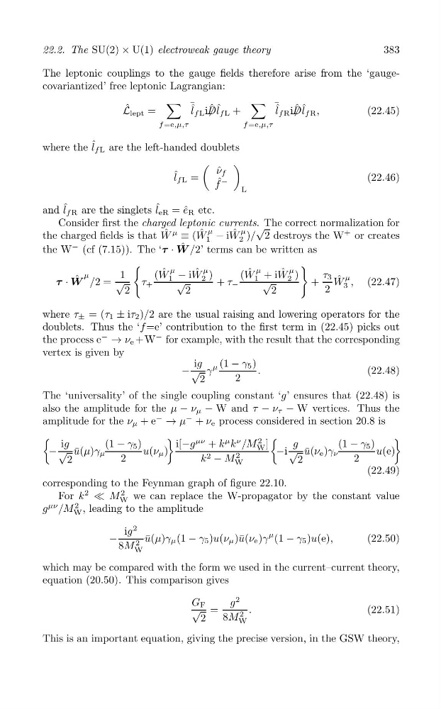
The leptonic couplings to the gauge fields therefore arise from the ‘gaugecovariantized’ free leptonic Lagrangian:
∑
∑
¯
¯
L ˆ
ˆ ˆ ˆ
ˆ ˆ ˆ
lept =
l f L iDl f L +
l f R iDl f R ,
(22.45)
f =e,μ,τ
f =e,μ,τ
ˆ
where the l f L are the left-handed doublets
(
)
ν ˆ
ˆ
f
l f L =
(22.46)
ˆ
f
−
L
ˆ
ˆ
and l f R are the singlets l eR = ˆ
e R etc.
Consider first the charged leptonic currents. The correct normalization for
ˆ
ˆ μ
ˆ μ
the charged fields is that W
μ
≡ (W 1 − iW 2 )/
√
2 destroys the W
+ or creates
the W
− (cf (7.15)). The ‘τ · ˆ
W /2’ terms can be written as
(
(
μ
μ
ˆ μ
μ
ˆ
ˆ
ˆ
1
(W 1 −
μ
iW )
W /2 = √
2
(W + i
τ
· ˆ
τ
2
√
+ τ
1
W )
τ +
2
−
√
2
3 ˆ μ
+ W
2
2
3 , (22.47)
where τ = (τ 1 ± iτ 2 )/2 are the usual raising and lowering operators for the
±
doublets. Thus the ‘f =e’ contribution to the first term in (22.45) picks out
the process e
−
→ ν e +W
− for example, with the result that the corresponding
vertex is given by
ig
− √ γ
μ (1 − γ 5 ) .
(22.48)
2
2
The ‘universality’ of the single coupling constant ‘g’ ensures that (22.48) is
also the amplitude for the μ − ν μ − W and τ − ν τ − W vertices. Thus the
amplitude for the ν μ + e
−
→ μ
− + ν e process considered in section 20.8 is
(
)
μν
μ ν
2
(
)
ig
(1 γ )
i[ g + k k /M
√
5
u ¯(μ)γ
W ]
g
(1 γ 5 )
−
μ
−
u(ν μ )
−
ν
2
k − M 2
W
−i √ u ¯( e )γ ν
2
−
u(e)
2
2
2
(22.49)
corresponding to the Feynman graph of figure 22.10.
For k
2
≪ M
2
W we can replace the W-propagator by the constant value
g
μν /M
2
W , leading to the amplitude
ig
2
−
u ¯(μ)γ
μ
μ (1 − γ 5 )u(ν μ )¯ u(ν e )γ (1 − γ 5 )u(e),
(22.50)
8M 2
W
which may be compared with the form we used in the current–current theory,
equation (20.50). This comparison gives
G
√
F
g
2
=
.
(22.51)
2
8M 2
W
This is an important equation, giving the precise version, in the GSW theory,
/
/
383
The leptonic couplings to the gauge fields therefore arise from the ‘gaugecovariantized’ free leptonic Lagrangian:
∑
∑
¯
¯
L ˆ
ˆ ˆ ˆ
ˆ ˆ ˆ
lept =
l f L iDl f L +
l f R iDl f R ,
(22.45)
f =e,μ,τ
f =e,μ,τ
ˆ
where the l f L are the left-handed doublets
(
)
ν ˆ
ˆ
f
l f L =
(22.46)
ˆ
f
−
L
ˆ
ˆ
and l f R are the singlets l eR = ˆ
e R etc.
Consider first the charged leptonic currents. The correct normalization for
ˆ
ˆ μ
ˆ μ
the charged fields is that W
μ
≡ (W 1 − iW 2 )/
√
2 destroys the W
+ or creates
the W
− (cf (7.15)). The ‘τ · ˆ
W /2’ terms can be written as
(
(
μ
μ
ˆ μ
μ
ˆ
ˆ
ˆ
1
(W 1 −
μ
iW )
W /2 = √
2
(W + i
τ
· ˆ
τ
2
√
+ τ
1
W )
τ +
2
−
√
2
3 ˆ μ
+ W
2
2
3 , (22.47)
where τ = (τ 1 ± iτ 2 )/2 are the usual raising and lowering operators for the
±
doublets. Thus the ‘f =e’ contribution to the first term in (22.45) picks out
the process e
−
→ ν e +W
− for example, with the result that the corresponding
vertex is given by
ig
− √ γ
μ (1 − γ 5 ) .
(22.48)
2
2
The ‘universality’ of the single coupling constant ‘g’ ensures that (22.48) is
also the amplitude for the μ − ν μ − W and τ − ν τ − W vertices. Thus the
amplitude for the ν μ + e
−
→ μ
− + ν e process considered in section 20.8 is
(
)
μν
μ ν
2
(
)
ig
(1 γ )
i[ g + k k /M
√
5
u ¯(μ)γ
W ]
g
(1 γ 5 )
−
μ
−
u(ν μ )
−
ν
2
k − M 2
W
−i √ u ¯( e )γ ν
2
−
u(e)
2
2
2
(22.49)
corresponding to the Feynman graph of figure 22.10.
For k
2
≪ M
2
W we can replace the W-propagator by the constant value
g
μν /M
2
W , leading to the amplitude
ig
2
−
u ¯(μ)γ
μ
μ (1 − γ 5 )u(ν μ )¯ u(ν e )γ (1 − γ 5 )u(e),
(22.50)
8M 2
W
which may be compared with the form we used in the current–current theory,
equation (20.50). This comparison gives
G
√
F
g
2
=
.
(22.51)
2
8M 2
W
This is an important equation, giving the precise version, in the GSW theory,
/
/