

382
22. The GSW Gauge Theory of Electroweak Interactions
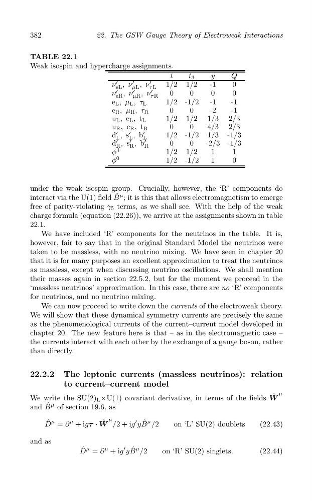
TABLE 22.1
Weak isospin and hypercharge assignments.
t
t 3
y
Q
′
′
′
ν , ν , ν
1/2 1/2
-1
0
eL
μL
τ L
′
′
′
ν , ν , ν
0
0
0
0
eR
μR
τ R
e L , μ L , τ L
1/2 -1/2 -1
-1
e R , μ R , τ R
0
0
-2
-1
u L , c L , t L
1/2 1/2 1/3 2/3
u R , c R , t R
0
0
4/3 2/3
d
′
′
L , s L , b
′
1/2 -1/2 1/3 -1/3
L
d
′
′
R , s R , b
′
0
0
-2/3 -1/3
R
+
φ
1/2 1/2
1
1
0
φ
1/2 -1/2
1
0
under the weak isospin group. Crucially, however, the ‘R’ components do
interact via the U(1) field B ˆ μ ; it is this that allows electromagnetism to emerge
free of parity-violating γ 5 terms, as we shall see. With the help of the weak
charge formula (equation (22.26)), we arrive at the assignments shown in table
22.1.
We have included ‘R’ components for the neutrinos in the table. It is,
however, fair to say that in the original Standard Model the neutrinos were
taken to be massless, with no neutrino mixing. We have seen in chapter 20
that it is for many purposes an excellent approximation to treat the neutrinos
as massless, except when discussing neutrino oscillations. We shall mention
their masses again in section 22.5.2, but for the moment we proceed in the
‘massless neutrinos’ approximation. In this case, there are no ‘R’ components
for neutrinos, and no neutrino mixing.
We can now proceed to write down the currents of the electroweak theory.
We will show that these dynamical symmetry currents are precisely the same
as the phenomenological currents of the current–current model developed in
chapter 20. The new feature here is that – as in the electromagnetic case –
the currents interact with each other by the exchange of a gauge boson, rather
than directly.
We write the SU(2) L ×U(1) covariant derivative, in terms of the fields ˆ
22.2.2 The leptonic currents (massless neutrinos): relation
to current–current model
μ
W
μ
and B ˆ of section 19.6, as
μ
μ
′
D ˆ = ∂
μ + igτ · W ˆ /2 + ig yB ˆ μ /2
on ‘L’ SU(2) doublets
(22.43)
and as
μ
′
D ˆ = ∂
μ + ig yB ˆ μ /2
on ‘R’ SU(2) singlets.
(22.44)
22. The GSW Gauge Theory of Electroweak Interactions
TABLE 22.1
Weak isospin and hypercharge assignments.
t
t 3
y
Q
′
′
′
ν , ν , ν
1/2 1/2
-1
0
eL
μL
τ L
′
′
′
ν , ν , ν
0
0
0
0
eR
μR
τ R
e L , μ L , τ L
1/2 -1/2 -1
-1
e R , μ R , τ R
0
0
-2
-1
u L , c L , t L
1/2 1/2 1/3 2/3
u R , c R , t R
0
0
4/3 2/3
d
′
′
L , s L , b
′
1/2 -1/2 1/3 -1/3
L
d
′
′
R , s R , b
′
0
0
-2/3 -1/3
R
+
φ
1/2 1/2
1
1
0
φ
1/2 -1/2
1
0
under the weak isospin group. Crucially, however, the ‘R’ components do
interact via the U(1) field B ˆ μ ; it is this that allows electromagnetism to emerge
free of parity-violating γ 5 terms, as we shall see. With the help of the weak
charge formula (equation (22.26)), we arrive at the assignments shown in table
22.1.
We have included ‘R’ components for the neutrinos in the table. It is,
however, fair to say that in the original Standard Model the neutrinos were
taken to be massless, with no neutrino mixing. We have seen in chapter 20
that it is for many purposes an excellent approximation to treat the neutrinos
as massless, except when discussing neutrino oscillations. We shall mention
their masses again in section 22.5.2, but for the moment we proceed in the
‘massless neutrinos’ approximation. In this case, there are no ‘R’ components
for neutrinos, and no neutrino mixing.
We can now proceed to write down the currents of the electroweak theory.
We will show that these dynamical symmetry currents are precisely the same
as the phenomenological currents of the current–current model developed in
chapter 20. The new feature here is that – as in the electromagnetic case –
the currents interact with each other by the exchange of a gauge boson, rather
than directly.
We write the SU(2) L ×U(1) covariant derivative, in terms of the fields ˆ
22.2.2 The leptonic currents (massless neutrinos): relation
to current–current model
μ
W
μ
and B ˆ of section 19.6, as
μ
μ
′
D ˆ = ∂
μ + igτ · W ˆ /2 + ig yB ˆ μ /2
on ‘L’ SU(2) doublets
(22.43)
and as
μ
′
D ˆ = ∂
μ + ig yB ˆ μ /2
on ‘R’ SU(2) singlets.
(22.44)