

251
18.4. Chiral anomalies
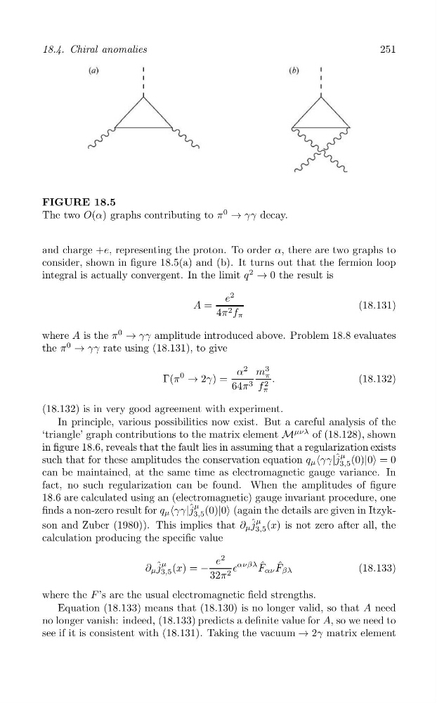
FIGURE 18.5
The two O(α) graphs contributing to π
0
→ γγ decay.
and charge +e, representing the proton. To order α, there are two graphs to
consider, shown in figure 18.5(a) and (b). It turns out that the fermion loop
integral is actually convergent. In the limit q
2
→ 0 the result is
2
e
A =
(18.131)
4π 2 f π
where A is the π
0
→ γγ amplitude introduced above. Problem 18.8 evaluates
the π
0
→ γγ rate using (18.131), to give
α
2 m
3
π
Γ(π
0
→ 2γ) =
f 2 .
(18.132)
64π 3
π
(18.132) is in very good agreement with experiment.
In principle, various possibilities now exist. But a careful analysis of the
‘triangle’ graph contributions to the matrix element M
μνλ of (18.128), shown
in figure 18.6, reveals that the fault lies in assuming that a regularization exists
μ
such that for these amplitudes the conservation equation q μ ‹γγ| ˆ j (0)|0› = 0
3,5
can be maintained, at the same time as electromagnetic gauge variance. In
fact, no such regularization can be found. When the amplitudes of figure
18.6 are calculated using an (electromagnetic) gauge invariant procedure, one
μ
finds a non-zero result for q μ ‹γγ| ˆ j (0)|0› (again the details are given in Itzyk3,5
μ
ˆ
son and Zuber (1980)). This implies that ∂ μ j 3,5 (x) is not zero after all, the
calculation producing the specific value
2
e
ˆ μ
∈
ανβλ ˆ ˆ
∂ μ j 3,5 (x) = −
F αν F βλ
(18.133)
32π 2
where the F ’s are the usual electromagnetic field strengths.
Equation (18.133) means that (18.130) is no longer valid, so that A need
no longer vanish: indeed, (18.133) predicts a definite value for A, so we need to
see if it is consistent with (18.131). Taking the vacuum → 2γ matrix element