

250
18. Chiral Symmetry Breaking
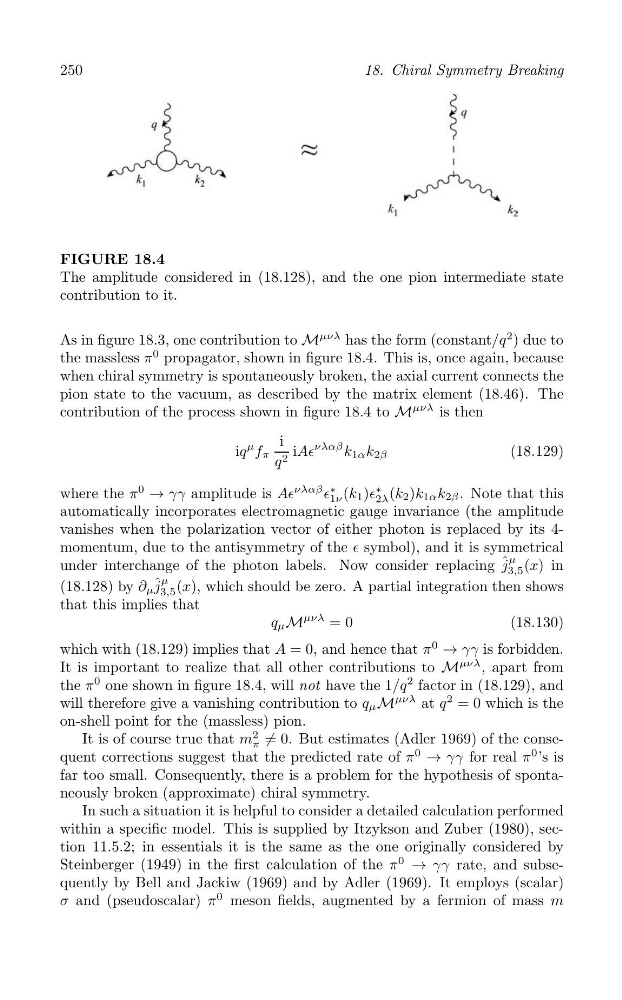
FIGURE 18.4
The amplitude considered in (18.128), and the one pion intermediate state
contribution to it.
As in figure 18.3, one contribution to M
μνλ has the form (constant/q
2 ) due to
the massless π
0 propagator, shown in figure 18.4. This is, once again, because
when chiral symmetry is spontaneously broken, the axial current connects the
pion state to the vacuum, as described by the matrix element (18.46). The
contribution of the process shown in figure 18.4 to M
μνλ is then
iA∈
νλαβ k 1α k 2β
iq
μ f π q
i
2
(18.129)
where the π
0
→ γγ amplitude is A∈
νλαβ ∈
∗ (k 1 )∈
∗ (k 2 )k 1α k 2β . Note that this
1ν
2λ
automatically incorporates electromagnetic gauge invariance (the amplitude
vanishes when the polarization vector of either photon is replaced by its 4momentum, due to the antisymmetry of the ∈ symbol), and it is symmetrical
μ
under interchange of the photon labels. Now consider replacing ˆ j (x) in
3,5
μ
ˆ
(18.128) by ∂ μ j (x), which should be zero. A partial integration then shows
3,5
that this implies that
q μ M
μνλ = 0
(18.130)
which with (18.129) implies that A = 0, and hence that π
0
→ γγ is forbidden.
It is important to realize that all other contributions to M
μνλ , apart from
the π
0 one shown in figure 18.4, will not have the 1/q
2 factor in (18.129), and
will therefore give a vanishing contribution to q μ M
μνλ at q
2 = 0 which is the
on-shell point for the (massless) pion.
2
It is of course true that m / 0. But estimates (Adler 1969) of the conse=
π
quent corrections suggest that the predicted rate of π
0
→ γγ for real π
0 ’s is
far too small. Consequently, there is a problem for the hypothesis of spontaneously broken (approximate) chiral symmetry.
In such a situation it is helpful to consider a detailed calculation performed
within a specific model. This is supplied by Itzykson and Zuber (1980), section 11.5.2; in essentials it is the same as the one originally considered by
Steinberger (1949) in the first calculation of the π
0
→ γγ rate, and subsequently by Bell and Jackiw (1969) and by Adler (1969). It employs (scalar)
σ and (pseudoscalar) π
0 meson fields, augmented by a fermion of mass m