

15.6. QCD corrections to the parton model predictions: scaling violations 147
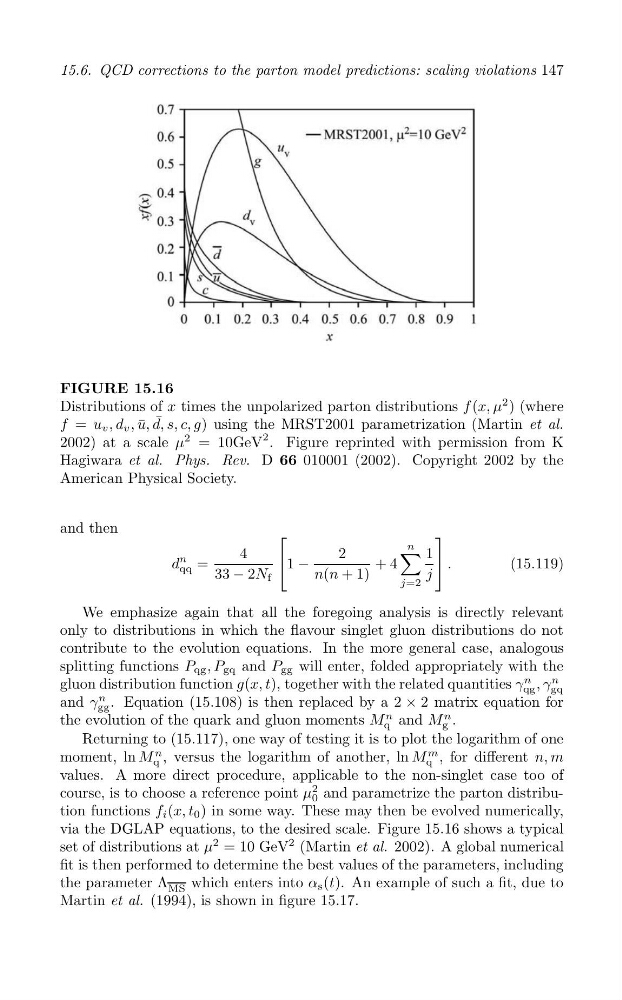
FIGURE 15.16
Distributions of x times the unpolarized parton distributions f (x, μ
2 ) (where
¯
f = u v , d v , u, ¯ d, s, c, g) using the MRST2001 parametrization (Martin et al.
2002) at a scale μ
2 = 10GeV
2 . Figure reprinted with permission from K
Hagiwara et al. Phys. Rev. D 66 010001 (2002). Copyright 2002 by the
American Physical Society.
and then
[
]
n
∑
4
2
1
d
n
| 1 −
|
qq =
+ 4
.
(15.119)
33 − 2N f
n(n + 1)
j
j=2
We emphasize again that all the foregoing analysis is directly relevant
only to distributions in which the flavour singlet gluon distributions do not
contribute to the evolution equations. In the more general case, analogous
splitting functions P qg , P gq and P gg will enter, folded appropriately with the
gluon distribution function g(x, t), together with the related quantities γ
n , γ
n
qg gq
and γ
n . Equation (15.108) is then replaced by a 2 × 2 matrix equation for
gg
the evolution of the quark and gluon moments M
n and M
n .
q
g
Returning to (15.117), one way of testing it is to plot the logarithm of one
moment, ln M
n , versus the logarithm of another, ln M
m , for different n, m
q
q
values. A more direct procedure, applicable to the non-singlet case too of
course, is to choose a reference point μ
2 and parametrize the parton distribu0
tion functions f i (x, t 0 ) in some way. These may then be evolved numerically,
via the DGLAP equations, to the desired scale. Figure 15.16 shows a typical
set of distributions at μ
2 = 10 GeV
2 (Martin et al. 2002). A global numerical
fit is then performed to determine the best values of the parameters, including
the parameter Λ
which enters into α s (t). An example of such a fit, due to
MS
Martin et al. (1994), is shown in figure 15.17.