

146
15. QCD II: Asymptotic Freedom, the Renormalization Group
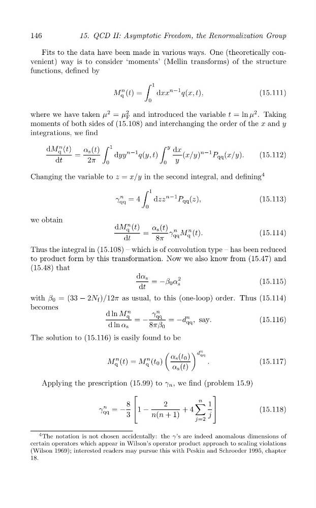
Fits to the data have been made in various ways. One (theoretically convenient) way is to consider ‘moments’ (Mellin transforms) of the structure
functions, defined by
∫ 1
M
n
q (t) =
dxx
n−1 q(x, t),
(15.111)
0
where we have taken μ
2 = μ
2
F and introduced the variable t = ln μ
2 . Taking
moments of both sides of (15.108) and interchanging the order of the x and y
integrations, we find
dM
n
∫
∫
q (t)
α s (t)
1
y
=
dyy
n
d
−1
x
q(y, t)
(x/y)
n−1 P qq (x/y).
(15.112)
dt
2π 0
0
y
Changing the variable to z = x/y in the second integral, and defining
4
∫ 1
γ
n
qq = 4
dzz
n−1 P qq (z),
(15.113)
0
we obtain
dM
n
q (t)
α s (t)
=
γ
n M
n (t).
(15.114)
dt
8π
qq q
Thus the integral in (15.108) – which is of convolution type – has been reduced
to product form by this transformation. Now we also know from (15.47) and
(15.48) that
dα s = −β 0 α
2
dt
s
(15.115)
with β 0 = (33 − 2N f )/12π as usual, to this (one-loop) order. Thus (15.114)
becomes
d ln M
n
n
q
γ qq
=
= d
n , say.
(15.116)
d ln α s
− 8πβ
− qq
0
The solution to (15.116) is easily found to be
(
) d
n
n
n
α s (t 0 )
qq
M q (t) = M q (t 0 )
.
(15.117)
α s (t)
Applying the prescription (15.99) to γ n , we find (problem 15.9)
[
]
n
n
8
2
∑
γ qq = − |
1
1
3
−
+ 4
|
(15.118)
n(n + 1)
j
j=2
4 The notation is not chosen accidentally: the γ’s are indeed anomalous dimensions of
certain operators which appear in Wilson’s operator product approach to scaling violations
(Wilson 1969); interested readers may pursue this with Peskin and Schroeder 1995, chapter
18.
15. QCD II: Asymptotic Freedom, the Renormalization Group
Fits to the data have been made in various ways. One (theoretically convenient) way is to consider ‘moments’ (Mellin transforms) of the structure
functions, defined by
∫ 1
M
n
q (t) =
dxx
n−1 q(x, t),
(15.111)
0
where we have taken μ
2 = μ
2
F and introduced the variable t = ln μ
2 . Taking
moments of both sides of (15.108) and interchanging the order of the x and y
integrations, we find
dM
n
∫
∫
q (t)
α s (t)
1
y
=
dyy
n
d
−1
x
q(y, t)
(x/y)
n−1 P qq (x/y).
(15.112)
dt
2π 0
0
y
Changing the variable to z = x/y in the second integral, and defining
4
∫ 1
γ
n
qq = 4
dzz
n−1 P qq (z),
(15.113)
0
we obtain
dM
n
q (t)
α s (t)
=
γ
n M
n (t).
(15.114)
dt
8π
qq q
Thus the integral in (15.108) – which is of convolution type – has been reduced
to product form by this transformation. Now we also know from (15.47) and
(15.48) that
dα s = −β 0 α
2
dt
s
(15.115)
with β 0 = (33 − 2N f )/12π as usual, to this (one-loop) order. Thus (15.114)
becomes
d ln M
n
n
q
γ qq
=
= d
n , say.
(15.116)
d ln α s
− 8πβ
0
The solution to (15.116) is easily found to be
(
) d
n
n
n
α s (t 0 )
M q (t) = M q (t 0 )
.
(15.117)
α s (t)
Applying the prescription (15.99) to γ n , we find (problem 15.9)
[
]
n
n
8
2
∑
γ qq = − |
1
1
3
−
+ 4
|
(15.118)
n(n + 1)
j
j=2
4 The notation is not chosen accidentally: the γ’s are indeed anomalous dimensions of
certain operators which appear in Wilson’s operator product approach to scaling violations
(Wilson 1969); interested readers may pursue this with Peskin and Schroeder 1995, chapter
18.