

64
13. Local Non-Abelian (Gauge) Symmetries
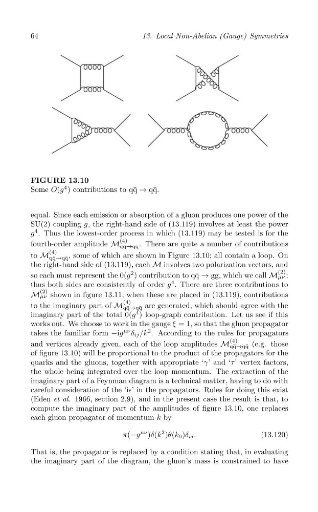
FIGURE 13.10
Some O(g
4 ) contributions to q¯ q → q¯ q.
equal. Since each emission or absorption of a gluon produces one power of the
SU(2) coupling g, the right-hand side of (13.119) involves at least the power
g
4 . Thus the lowest-order process in which (13.119) may be tested is for the
(4)
fourth-order amplitude M
. There are quite a number of contributions
q¯ q→q¯ q
(4)
to M
, some of which are shown in Figure 13.10; all contain a loop. On
q¯ q→q¯ q
the right-hand side of (13.119), each M involves two polarization vectors, and
(2)
so each must represent the 0(g
2 ) contribution to q¯ q → gg, which we call M μν ;
thus both sides are consistently of order g
4 . There are three contributions to
(2)
M μν shown in figure 13.11; when these are placed in (13.119), contributions
(4)
to the imaginary part of M
are generated, which should agree with the
q¯ q→q¯ q
imaginary part of the total 0(g
4 ) loop-graph contribution. Let us see if this
works out. We choose to work in the gauge ξ = 1, so that the gluon propagator
takes the familiar form −ig
μν δ ij /k
2 . According to the rules for propagators
(4)
and vertices already given, each of the loop amplitudes M
(e.g. those
q¯ q→q¯ q
of figure 13.10) will be proportional to the product of the propagators for the
quarks and the gluons, together with appropriate ‘γ’ and ‘τ ’ vertex factors,
the whole being integrated over the loop momentum. The extraction of the
imaginary part of a Feynman diagram is a technical matter, having to do with
careful consideration of the ‘i∈’ in the propagators. Rules for doing this exist
(Eden et al. 1966, section 2.9), and in the present case the result is that, to
compute the imaginary part of the amplitudes of figure 13.10, one replaces
each gluon propagator of momentum k by
π(−g
μν )δ(k
2 )θ(k 0 )δ ij .
(13.120)
That is, the propagator is replaced by a condition stating that, in evaluating
the imaginary part of the diagram, the gluon’s mass is constrained to have
13. Local Non-Abelian (Gauge) Symmetries
FIGURE 13.10
Some O(g
4 ) contributions to q¯ q → q¯ q.
equal. Since each emission or absorption of a gluon produces one power of the
SU(2) coupling g, the right-hand side of (13.119) involves at least the power
g
4 . Thus the lowest-order process in which (13.119) may be tested is for the
(4)
fourth-order amplitude M
. There are quite a number of contributions
q¯ q→q¯ q
(4)
to M
, some of which are shown in Figure 13.10; all contain a loop. On
q¯ q→q¯ q
the right-hand side of (13.119), each M involves two polarization vectors, and
(2)
so each must represent the 0(g
2 ) contribution to q¯ q → gg, which we call M μν ;
thus both sides are consistently of order g
4 . There are three contributions to
(2)
M μν shown in figure 13.11; when these are placed in (13.119), contributions
(4)
to the imaginary part of M
are generated, which should agree with the
q¯ q→q¯ q
imaginary part of the total 0(g
4 ) loop-graph contribution. Let us see if this
works out. We choose to work in the gauge ξ = 1, so that the gluon propagator
takes the familiar form −ig
μν δ ij /k
2 . According to the rules for propagators
(4)
and vertices already given, each of the loop amplitudes M
(e.g. those
q¯ q→q¯ q
of figure 13.10) will be proportional to the product of the propagators for the
quarks and the gluons, together with appropriate ‘γ’ and ‘τ ’ vertex factors,
the whole being integrated over the loop momentum. The extraction of the
imaginary part of a Feynman diagram is a technical matter, having to do with
careful consideration of the ‘i∈’ in the propagators. Rules for doing this exist
(Eden et al. 1966, section 2.9), and in the present case the result is that, to
compute the imaginary part of the amplitudes of figure 13.10, one replaces
each gluon propagator of momentum k by
π(−g
μν )δ(k
2 )θ(k 0 )δ ij .
(13.120)
That is, the propagator is replaced by a condition stating that, in evaluating
the imaginary part of the diagram, the gluon’s mass is constrained to have