

60
13. Local Non-Abelian (Gauge) Symmetries
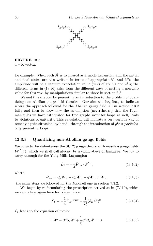
FIGURE 13.8
4 − X vertex.
for example. When each X ˆ is expressed as a mode expansion, and the initial
and final states are also written in terms of appropriate ˆ
a’s and ˆ
a
† ’s, the
amplitude will be a vacuum expectation value (vev) of six ˆ
a’s and ˆ
a
† ’s; the
different terms in (13.96) arise from the different ways of getting a non-zero
value for this vev, by manipulations similar to those in section 6.3.
We end this chapter by presenting an introduction to the problem of quantizing non-Abelian gauge field theories. Our aim will be, first, to indicate
where the approach followed for the Abelian gauge field A ˆ μ in section 7.3.2
fails; and then to show how the assumption (nevertheless) that the Feynman rules we have established for tree graphs work for loops as well, leads
to violations of unitarity. This calculation will indicate a very curious way of
remedying the situation ‘by hand’, through the introduction of ghost particles,
only present in loops.
13.3.3
Quantizing non-Abelian gauge fields
We consider for definiteness the SU(2) gauge theory with massless gauge fields
μ
ˆ
W (x), which we shall call gluons, by a slight abuse of language. We try to
carry through for the Yang-Mills Lagrangian
1
μν
ˆ
ˆ
ˆ
L 2 = − F μν · F ,
(13.102)
4
where
ˆ
ˆ
ˆ
=
W ˆ μ − gW μ × ˆ
(13.103)
the same steps we followed for the Maxwell one in section 7.3.2.
We begin by re-formulating the prescription arrived at in (7.119), which
we reproduce again here for convenience:
F μν ∂ μ W ν − ∂ ν
W ν ,
ˆ F ˆ μν −
ˆ
L ˆ ξ = −
1 F μν
1 (∂ μ A
μ )
2 .
(13.104)
4
2ξ
ˆ
L ξ leads to the equation of motion
❗A ˆ μ − ∂
μ ∂ ν A ˆ ν 1 ∂
μ ∂ ν A ˆ ν = 0.
(13.105)
+ ξ
13. Local Non-Abelian (Gauge) Symmetries
FIGURE 13.8
4 − X vertex.
for example. When each X ˆ is expressed as a mode expansion, and the initial
and final states are also written in terms of appropriate ˆ
a’s and ˆ
a
† ’s, the
amplitude will be a vacuum expectation value (vev) of six ˆ
a’s and ˆ
a
† ’s; the
different terms in (13.96) arise from the different ways of getting a non-zero
value for this vev, by manipulations similar to those in section 6.3.
We end this chapter by presenting an introduction to the problem of quantizing non-Abelian gauge field theories. Our aim will be, first, to indicate
where the approach followed for the Abelian gauge field A ˆ μ in section 7.3.2
fails; and then to show how the assumption (nevertheless) that the Feynman rules we have established for tree graphs work for loops as well, leads
to violations of unitarity. This calculation will indicate a very curious way of
remedying the situation ‘by hand’, through the introduction of ghost particles,
only present in loops.
13.3.3
Quantizing non-Abelian gauge fields
We consider for definiteness the SU(2) gauge theory with massless gauge fields
μ
ˆ
W (x), which we shall call gluons, by a slight abuse of language. We try to
carry through for the Yang-Mills Lagrangian
1
μν
ˆ
ˆ
ˆ
L 2 = − F μν · F ,
(13.102)
4
where
ˆ
ˆ
ˆ
=
W ˆ μ − gW μ × ˆ
(13.103)
the same steps we followed for the Maxwell one in section 7.3.2.
We begin by re-formulating the prescription arrived at in (7.119), which
we reproduce again here for convenience:
F μν ∂ μ W ν − ∂ ν
W ν ,
ˆ F ˆ μν −
ˆ
L ˆ ξ = −
1 F μν
1 (∂ μ A
μ )
2 .
(13.104)
4
2ξ
ˆ
L ξ leads to the equation of motion
❗A ˆ μ − ∂
μ ∂ ν A ˆ ν 1 ∂
μ ∂ ν A ˆ ν = 0.
(13.105)
+ ξ