

13.3. Local non-Abelian symmetries in Lagrangian quantum field theory 59
γ
γ
X
X
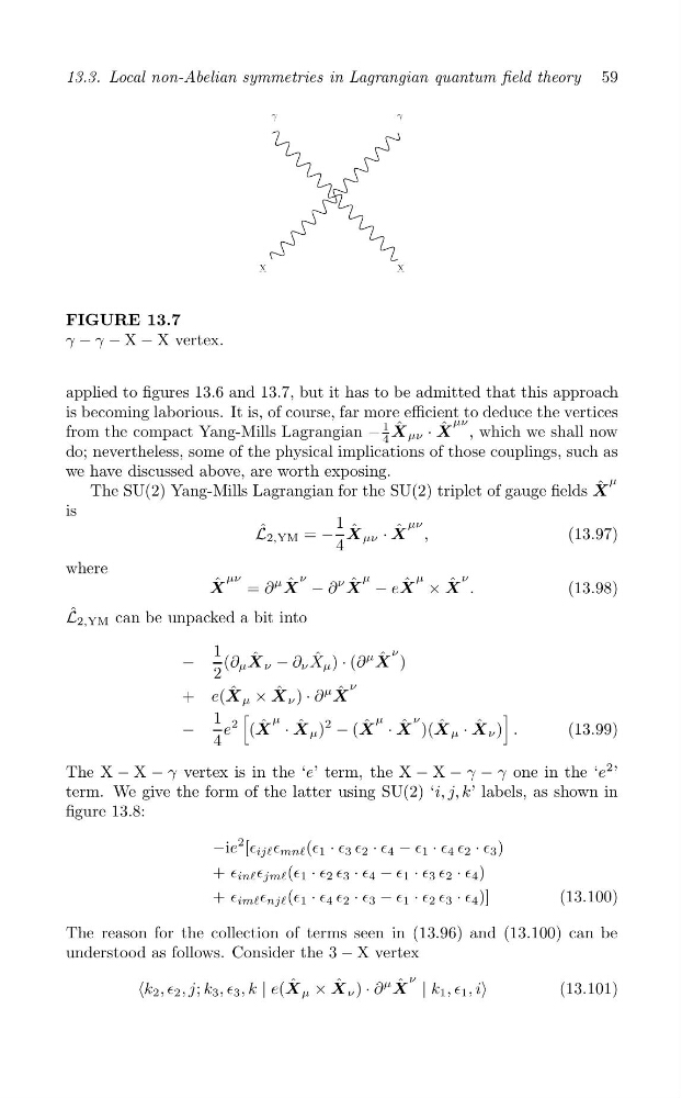
FIGURE 13.7
γ − γ − X − X vertex.
applied to figures 13.6 and 13.7, but it has to be admitted that this approach
is becoming laborious. It is, of course, far more efficient to deduce the vertices
μν
from the compact Yang-Mills Lagrangian −
1
X ˆ μν · X ˆ , which we shall now
4
do; nevertheless, some of the physical implications of those couplings, such as
we have discussed above, are worth exposing.
μ
The SU(2) Yang-Mills Lagrangian for the SU(2) triplet of gauge fields X ˆ
is
1
μν
ˆ
ˆ · ˆ
L 2,YM = − X μν X ,
(13.97)
4
where
μν
ν
μ
μ
ν
ˆ
∂
μ ˆ − ∂
ν ˆ
ˆ × ˆ
X = X
X − eX
X .
(13.98)
ˆ
L 2,YM can be unpacked a bit into
−
1 (∂ μ X ˆ ν − ∂ ν X ˆ μ ) · (∂
μ
X ˆ
ν
)
2
ν
+ e(X ˆ μ × X ˆ ν ) · ∂
μ
X ˆ
[
]
1
μ
μ
ν
2
−
e (X ˆ · X ˆ μ )
2
− (X ˆ · X ˆ )(X ˆ μ · X ˆ ν ) .
(13.99)
4
The X − X − γ vertex is in the ‘e’ term, the X − X − γ − γ one in the ‘e
2 ’
term. We give the form of the latter using SU(2) ‘i, j, k’ labels, as shown in
figure 13.8:
−ie
2 [∈ ije ∈ mne (∈ 1 · ∈ 3 ∈ 2 · ∈ 4 − ∈ 1 · ∈ 4 ∈ 2 · ∈ 3 )
+ ∈ ine ∈ jme (∈ 1 · ∈ 2 ∈ 3 · ∈ 4 − ∈ 1 · ∈ 3 ∈ 2 · ∈ 4 )
+ ∈ ime ∈ nje (∈ 1 · ∈ 4 ∈ 2 · ∈ 3 − ∈ 1 · ∈ 2 ∈ 3 · ∈ 4 )]
(13.100)
The reason for the collection of terms seen in (13.96) and (13.100) can be
understood as follows. Consider the 3 − X vertex
ν
‹k 2 , ∈ 2 , j; k 3 , ∈ 3 , k | e(X ˆ μ × X ˆ ν ) · ∂
μ
X ˆ | k 1 , ∈ 1 , i›
(13.101)
γ
γ
X
X
FIGURE 13.7
γ − γ − X − X vertex.
applied to figures 13.6 and 13.7, but it has to be admitted that this approach
is becoming laborious. It is, of course, far more efficient to deduce the vertices
μν
from the compact Yang-Mills Lagrangian −
1
X ˆ μν · X ˆ , which we shall now
4
do; nevertheless, some of the physical implications of those couplings, such as
we have discussed above, are worth exposing.
μ
The SU(2) Yang-Mills Lagrangian for the SU(2) triplet of gauge fields X ˆ
is
1
μν
ˆ
ˆ · ˆ
L 2,YM = − X μν X ,
(13.97)
4
where
μν
ν
μ
μ
ν
ˆ
∂
μ ˆ − ∂
ν ˆ
ˆ × ˆ
X = X
X − eX
X .
(13.98)
ˆ
L 2,YM can be unpacked a bit into
−
1 (∂ μ X ˆ ν − ∂ ν X ˆ μ ) · (∂
μ
X ˆ
ν
)
2
ν
+ e(X ˆ μ × X ˆ ν ) · ∂
μ
X ˆ
[
]
1
μ
μ
ν
2
−
e (X ˆ · X ˆ μ )
2
− (X ˆ · X ˆ )(X ˆ μ · X ˆ ν ) .
(13.99)
4
The X − X − γ vertex is in the ‘e’ term, the X − X − γ − γ one in the ‘e
2 ’
term. We give the form of the latter using SU(2) ‘i, j, k’ labels, as shown in
figure 13.8:
−ie
2 [∈ ije ∈ mne (∈ 1 · ∈ 3 ∈ 2 · ∈ 4 − ∈ 1 · ∈ 4 ∈ 2 · ∈ 3 )
+ ∈ ine ∈ jme (∈ 1 · ∈ 2 ∈ 3 · ∈ 4 − ∈ 1 · ∈ 3 ∈ 2 · ∈ 4 )
+ ∈ ime ∈ nje (∈ 1 · ∈ 4 ∈ 2 · ∈ 3 − ∈ 1 · ∈ 2 ∈ 3 · ∈ 4 )]
(13.100)
The reason for the collection of terms seen in (13.96) and (13.100) can be
understood as follows. Consider the 3 − X vertex
ν
‹k 2 , ∈ 2 , j; k 3 , ∈ 3 , k | e(X ˆ μ × X ˆ ν ) · ∂
μ
X ˆ | k 1 , ∈ 1 , i›
(13.101)