

58
13. Local Non-Abelian (Gauge) Symmetries
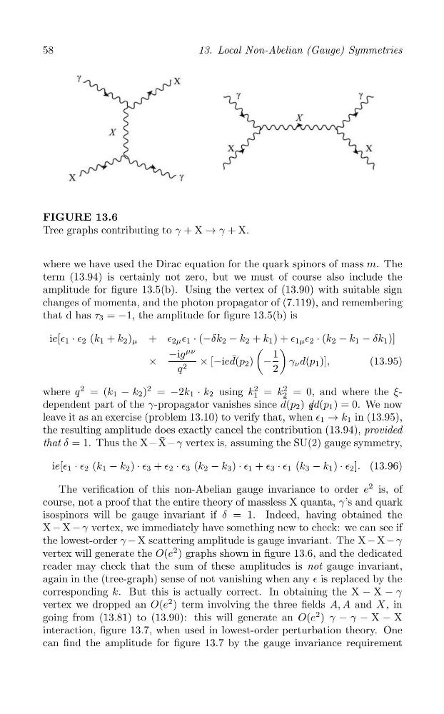
FIGURE 13.6
Tree graphs contributing to γ + X → γ + X.
where we have used the Dirac equation for the quark spinors of mass m. The
term (13.94) is certainly not zero, but we must of course also include the
amplitude for figure 13.5(b). Using the vertex of (13.90) with suitable sign
changes of momenta, and the photon propagator of (7.119), and remembering
that d has τ 3 = −1, the amplitude for figure 13.5(b) is
ie[∈ 1 · ∈ 2 (k 1 + k 2 ) μ + ∈ 2μ ∈ 1 · (−δk 2 − k 2 + k 1 ) + ∈ 1μ ∈ 2 · (k 2 − k 1 − δk 1 )]
)
(
μν
−ig
1
¯
×
× [−ied(p 2 ) −
γ ν d(p 1 )],
(13.95)
q 2
2
2
= k
2
where q = (k 1 − k 2 )
2 = −2k 1 · k 2 using k 1
2
2 = 0, and where the ξdependent part of the γ-propagator vanishes since d ¯ (p 2 ) / qd(p 1 ) = 0. We now
leave it as an exercise (problem 13.10) to verify that, when ∈ 1 → k 1 in (13.95),
the resulting amplitude does exactly cancel the contribution (13.94), provided
¯
that δ = 1. Thus the X− X− γ vertex is, assuming the SU(2) gauge symmetry,
ie[∈ 1 · ∈ 2 (k 1 − k 2 ) · ∈ 3 + ∈ 2 · ∈ 3 (k 2 − k 3 ) · ∈ 1 + ∈ 3 · ∈ 1 (k 3 − k 1 ) · ∈ 2 ]. (13.96)
2
The verification of this non-Abelian gauge invariance to order e is, of
course, not a proof that the entire theory of massless X quanta, γ’s and quark
isospinors will be gauge invariant if δ = 1. Indeed, having obtained the
X − X − γ vertex, we immediately have something new to check: we can see if
the lowest-order γ − X scattering amplitude is gauge invariant. The X − X − γ
vertex will generate the O(e
2 ) graphs shown in figure 13.6, and the dedicated
reader may check that the sum of these amplitudes is not gauge invariant,
again in the (tree-graph) sense of not vanishing when any ∈ is replaced by the
corresponding k. But this is actually correct. In obtaining the X − X − γ
vertex we dropped an O(e
2 ) term involving the three fields A, A and X, in
going from (13.81) to (13.90): this will generate an O(e
2 ) γ − γ − X − X
interaction, figure 13.7, when used in lowest-order perturbation theory. One
can find the amplitude for figure 13.7 by the gauge invariance requirement
13. Local Non-Abelian (Gauge) Symmetries
FIGURE 13.6
Tree graphs contributing to γ + X → γ + X.
where we have used the Dirac equation for the quark spinors of mass m. The
term (13.94) is certainly not zero, but we must of course also include the
amplitude for figure 13.5(b). Using the vertex of (13.90) with suitable sign
changes of momenta, and the photon propagator of (7.119), and remembering
that d has τ 3 = −1, the amplitude for figure 13.5(b) is
ie[∈ 1 · ∈ 2 (k 1 + k 2 ) μ + ∈ 2μ ∈ 1 · (−δk 2 − k 2 + k 1 ) + ∈ 1μ ∈ 2 · (k 2 − k 1 − δk 1 )]
)
(
μν
−ig
1
¯
×
× [−ied(p 2 ) −
γ ν d(p 1 )],
(13.95)
q 2
2
2
= k
2
where q = (k 1 − k 2 )
2 = −2k 1 · k 2 using k 1
2
2 = 0, and where the ξdependent part of the γ-propagator vanishes since d ¯ (p 2 ) / qd(p 1 ) = 0. We now
leave it as an exercise (problem 13.10) to verify that, when ∈ 1 → k 1 in (13.95),
the resulting amplitude does exactly cancel the contribution (13.94), provided
¯
that δ = 1. Thus the X− X− γ vertex is, assuming the SU(2) gauge symmetry,
ie[∈ 1 · ∈ 2 (k 1 − k 2 ) · ∈ 3 + ∈ 2 · ∈ 3 (k 2 − k 3 ) · ∈ 1 + ∈ 3 · ∈ 1 (k 3 − k 1 ) · ∈ 2 ]. (13.96)
2
The verification of this non-Abelian gauge invariance to order e is, of
course, not a proof that the entire theory of massless X quanta, γ’s and quark
isospinors will be gauge invariant if δ = 1. Indeed, having obtained the
X − X − γ vertex, we immediately have something new to check: we can see if
the lowest-order γ − X scattering amplitude is gauge invariant. The X − X − γ
vertex will generate the O(e
2 ) graphs shown in figure 13.6, and the dedicated
reader may check that the sum of these amplitudes is not gauge invariant,
again in the (tree-graph) sense of not vanishing when any ∈ is replaced by the
corresponding k. But this is actually correct. In obtaining the X − X − γ
vertex we dropped an O(e
2 ) term involving the three fields A, A and X, in
going from (13.81) to (13.90): this will generate an O(e
2 ) γ − γ − X − X
interaction, figure 13.7, when used in lowest-order perturbation theory. One
can find the amplitude for figure 13.7 by the gauge invariance requirement