

13.3. Local non-Abelian symmetries in Lagrangian quantum field theory 57
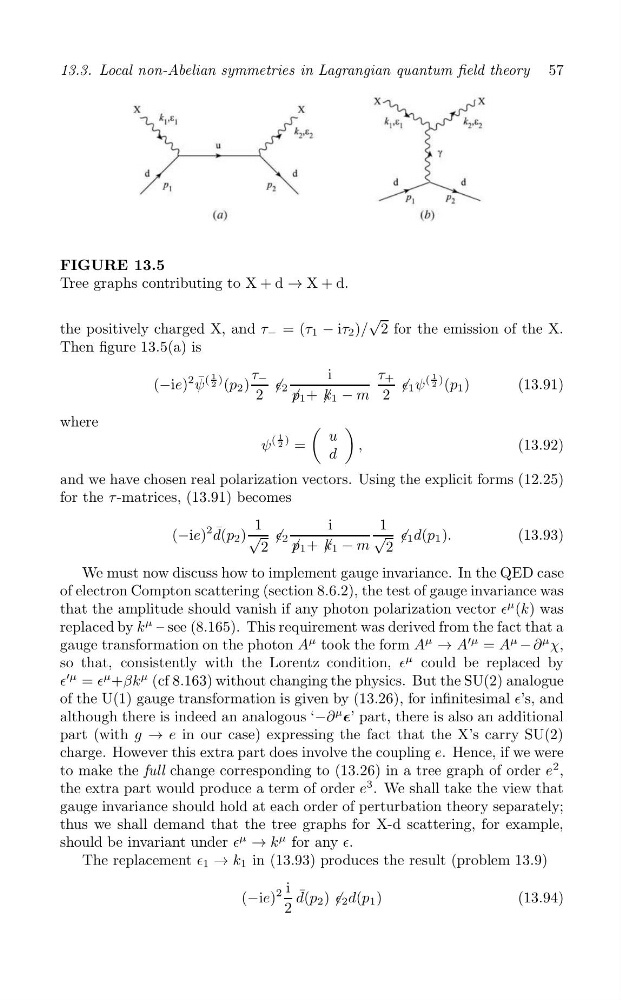
FIGURE 13.5
Tree graphs contributing to X + d → X + d.
√
the positively charged X, and τ − = (τ 1 − iτ 2 )/ 2 for the emission of the X.
Then figure 13.5(a) is
τ −
i
τ +
1
2
1
2
(−ie)
2 ψ ¯ ( ) (p 2 )
∈ 1 ψ
( ) (p 1 )
/
/
∈ 2
(13.91)
/ p 1 + / k 1 −
2
2
m
where
=
(
)
u
d
1
2
ψ
( )
(13.92)
,
and we have chosen real polarization vectors. Using the explicit forms (12.25)
for the τ -matrices, (13.91) becomes
1
i
1
(−ie)
2 d ¯ (p 2 ) √ / ∈ 2
√ / ∈ 1 d(p 1 ).
(13.93)
2 / p 1 + / k 1 − m 2
We must now discuss how to implement gauge invariance. In the QED case
of electron Compton scattering (section 8.6.2), the test of gauge invariance was
that the amplitude should vanish if any photon polarization vector ∈
μ (k) was
replaced by k
μ – see (8.165). This requirement was derived from the fact that a
gauge transformation on the photon A
μ took the form A
μ
→ A
′μ = A
μ
− ∂
μ χ,
so that, consistently with the Lorentz condition, ∈
μ could be replaced by
∈
′μ = ∈
μ +βk
μ (cf 8.163) without changing the physics. But the SU(2) analogue
of the U(1) gauge transformation is given by (13.26), for infinitesimal ∈’s, and
although there is indeed an analogous ‘−∂
μ
∊’ part, there is also an additional
part (with g → e in our case) expressing the fact that the X’s carry SU(2)
charge. However this extra part does involve the coupling e. Hence, if we were
to make the full change corresponding to (13.26) in a tree graph of order e ,
the extra part would produce a term of order e
3 . We shall take the view that
gauge invariance should hold at each order of perturbation theory separately;
thus we shall demand that the tree graphs for X-d scattering, for example,
should be invariant under ∈
μ
→ k
μ for any ∈.
The replacement ∈ 1 → k 1 in (13.93) produces the result (problem 13.9)
¯
(−ie)
2 i d(p 2 ) / ∈ 2 d(p 1 )
(13.94)
2
2
FIGURE 13.5
Tree graphs contributing to X + d → X + d.
√
the positively charged X, and τ − = (τ 1 − iτ 2 )/ 2 for the emission of the X.
Then figure 13.5(a) is
τ −
i
τ +
1
2
1
2
(−ie)
2 ψ ¯ ( ) (p 2 )
∈ 1 ψ
( ) (p 1 )
/
/
∈ 2
(13.91)
/ p 1 + / k 1 −
2
2
m
where
=
(
)
u
d
1
2
ψ
( )
(13.92)
,
and we have chosen real polarization vectors. Using the explicit forms (12.25)
for the τ -matrices, (13.91) becomes
1
i
1
(−ie)
2 d ¯ (p 2 ) √ / ∈ 2
√ / ∈ 1 d(p 1 ).
(13.93)
2 / p 1 + / k 1 − m 2
We must now discuss how to implement gauge invariance. In the QED case
of electron Compton scattering (section 8.6.2), the test of gauge invariance was
that the amplitude should vanish if any photon polarization vector ∈
μ (k) was
replaced by k
μ – see (8.165). This requirement was derived from the fact that a
gauge transformation on the photon A
μ took the form A
μ
→ A
′μ = A
μ
− ∂
μ χ,
so that, consistently with the Lorentz condition, ∈
μ could be replaced by
∈
′μ = ∈
μ +βk
μ (cf 8.163) without changing the physics. But the SU(2) analogue
of the U(1) gauge transformation is given by (13.26), for infinitesimal ∈’s, and
although there is indeed an analogous ‘−∂
μ
∊’ part, there is also an additional
part (with g → e in our case) expressing the fact that the X’s carry SU(2)
charge. However this extra part does involve the coupling e. Hence, if we were
to make the full change corresponding to (13.26) in a tree graph of order e ,
the extra part would produce a term of order e
3 . We shall take the view that
gauge invariance should hold at each order of perturbation theory separately;
thus we shall demand that the tree graphs for X-d scattering, for example,
should be invariant under ∈
μ
→ k
μ for any ∈.
The replacement ∈ 1 → k 1 in (13.93) produces the result (problem 13.9)
¯
(−ie)
2 i d(p 2 ) / ∈ 2 d(p 1 )
(13.94)
2
2