

56
13. Local Non-Abelian (Gauge) Symmetries
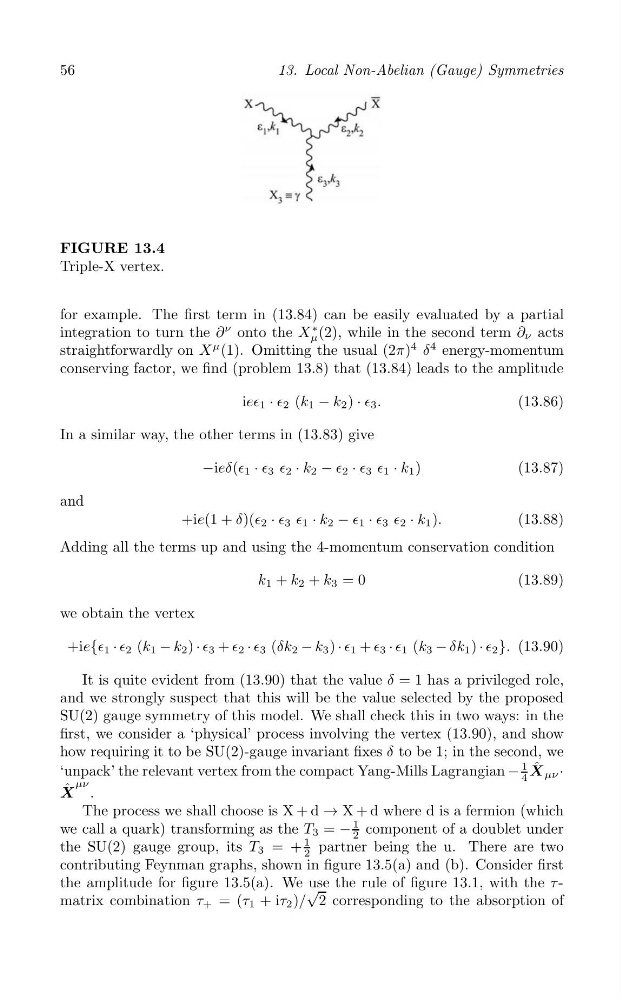
FIGURE 13.4
Triple-X vertex.
for example. The first term in (13.84) can be easily evaluated by a partial
integration to turn the ∂
ν onto the X
∗ (2), while in the second term ∂ ν acts
μ
straightforwardly on X
μ (1). Omitting the usual (2π)
4 δ
4 energy-momentum
conserving factor, we find (problem 13.8) that (13.84) leads to the amplitude
ie∈ 1 · ∈ 2 (k 1 − k 2 ) · ∈ 3 .
(13.86)
In a similar way, the other terms in (13.83) give
−ieδ(∈ 1 · ∈ 3 ∈ 2 · k 2 − ∈ 2 · ∈ 3 ∈ 1 · k 1 )
(13.87)
and
+ie(1 + δ)(∈ 2 · ∈ 3 ∈ 1 · k 2 − ∈ 1 · ∈ 3 ∈ 2 · k 1 ).
(13.88)
Adding all the terms up and using the 4-momentum conservation condition
k 1 + k 2 + k 3 = 0
(13.89)
we obtain the vertex
+ie{∈ 1 · ∈ 2 (k 1 − k 2 ) · ∈ 3 + ∈ 2 · ∈ 3 (δk 2 − k 3 ) · ∈ 1 + ∈ 3 · ∈ 1 (k 3 − δk 1 ) · ∈ 2 }. (13.90)
It is quite evident from (13.90) that the value δ = 1 has a privileged role,
and we strongly suspect that this will be the value selected by the proposed
SU(2) gauge symmetry of this model. We shall check this in two ways: in the
first, we consider a ‘physical’ process involving the vertex (13.90), and show
how requiring it to be SU(2)-gauge invariant fixes δ to be 1; in the second, we
‘unpack’ the relevant vertex from the compact Yang-Mills Lagrangian −
1
X ˆ μν ·
4
μν
ˆ
X .
The process we shall choose is X + d → X + d where d is a fermion (which
we call a quark) transforming as the T 3 = −
1 component of a doublet under
2
1
the SU(2) gauge group, its T 3 = + partner being the u. There are two
2
contributing Feynman graphs, shown in figure 13.5(a) and (b). Consider first
the amplitude for figure 13.5(a). We use the rule of figure 13.1, with the τ
√
matrix combination τ + = (τ 1 + iτ 2 )/ 2 corresponding to the absorption of
13. Local Non-Abelian (Gauge) Symmetries
FIGURE 13.4
Triple-X vertex.
for example. The first term in (13.84) can be easily evaluated by a partial
integration to turn the ∂
ν onto the X
∗ (2), while in the second term ∂ ν acts
μ
straightforwardly on X
μ (1). Omitting the usual (2π)
4 δ
4 energy-momentum
conserving factor, we find (problem 13.8) that (13.84) leads to the amplitude
ie∈ 1 · ∈ 2 (k 1 − k 2 ) · ∈ 3 .
(13.86)
In a similar way, the other terms in (13.83) give
−ieδ(∈ 1 · ∈ 3 ∈ 2 · k 2 − ∈ 2 · ∈ 3 ∈ 1 · k 1 )
(13.87)
and
+ie(1 + δ)(∈ 2 · ∈ 3 ∈ 1 · k 2 − ∈ 1 · ∈ 3 ∈ 2 · k 1 ).
(13.88)
Adding all the terms up and using the 4-momentum conservation condition
k 1 + k 2 + k 3 = 0
(13.89)
we obtain the vertex
+ie{∈ 1 · ∈ 2 (k 1 − k 2 ) · ∈ 3 + ∈ 2 · ∈ 3 (δk 2 − k 3 ) · ∈ 1 + ∈ 3 · ∈ 1 (k 3 − δk 1 ) · ∈ 2 }. (13.90)
It is quite evident from (13.90) that the value δ = 1 has a privileged role,
and we strongly suspect that this will be the value selected by the proposed
SU(2) gauge symmetry of this model. We shall check this in two ways: in the
first, we consider a ‘physical’ process involving the vertex (13.90), and show
how requiring it to be SU(2)-gauge invariant fixes δ to be 1; in the second, we
‘unpack’ the relevant vertex from the compact Yang-Mills Lagrangian −
1
X ˆ μν ·
4
μν
ˆ
X .
The process we shall choose is X + d → X + d where d is a fermion (which
we call a quark) transforming as the T 3 = −
1 component of a doublet under
2
1
the SU(2) gauge group, its T 3 = + partner being the u. There are two
2
contributing Feynman graphs, shown in figure 13.5(a) and (b). Consider first
the amplitude for figure 13.5(a). We use the rule of figure 13.1, with the τ
√
matrix combination τ + = (τ 1 + iτ 2 )/ 2 corresponding to the absorption of