

47
13.1. Local SU(2) symmetry
quantum number, so as to emphasize that it is not the hadronic isospin, for
which we retain T ; t will be the symbol used for the weak isospin to be
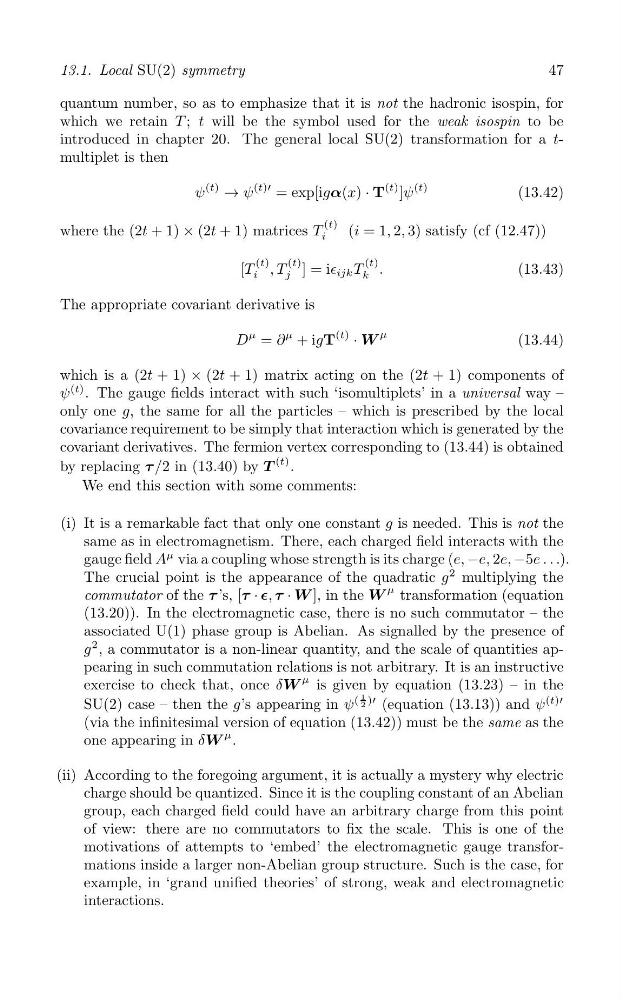
introduced in chapter 20. The general local SU(2) transformation for a tmultiplet is then
ψ
(t)
→ ψ
(t)′
T
(t) ]ψ
(t)
= exp[igα(x) ·
(13.42)
(t)
where the (2t + 1) × (2t + 1) matrices T
(i = 1, 2, 3) satisfy (cf (12.47))
i
(t)
(t)
(t)
[T , T ] = i∈ ijk T .
(13.43)
i
j
k
The appropriate covariant derivative is
D
μ = ∂
μ + igT
(t)
· W
μ
(13.44)
which is a (2t + 1) × (2t + 1) matrix acting on the (2t + 1) components of
ψ
(t) . The gauge fields interact with such ‘isomultiplets’ in a universal way –
only one g, the same for all the particles – which is prescribed by the local
covariance requirement to be simply that interaction which is generated by the
covariant derivatives. The fermion vertex corresponding to (13.44) is obtained
by replacing τ /2 in (13.40) by T
(t) .
We end this section with some comments:
(i) It is a remarkable fact that only one constant g is needed. This is not the
same as in electromagnetism. There, each charged field interacts with the
gauge field A
μ via a coupling whose strength is its charge (e, −e, 2e, −5e . . .).
2
The crucial point is the appearance of the quadratic g multiplying the
commutator of the τ ’s, [τ · ∊, τ · W ], in the W
μ transformation (equation
(13.20)). In the electromagnetic case, there is no such commutator – the
associated U(1) phase group is Abelian. As signalled by the presence of
g
2 , a commutator is a non-linear quantity, and the scale of quantities appearing in such commutation relations is not arbitrary. It is an instructive
exercise to check that, once δW
μ is given by equation (13.23) – in the
)′
2
SU(2) case – then the g’s appearing in ψ
(
1
(equation (13.13)) and ψ
(t)′
(via the infinitesimal version of equation (13.42)) must be the same as the
one appearing in δW
μ .
(ii) According to the foregoing argument, it is actually a mystery why electric
charge should be quantized. Since it is the coupling constant of an Abelian
group, each charged field could have an arbitrary charge from this point
of view: there are no commutators to fix the scale. This is one of the
motivations of attempts to ‘embed’ the electromagnetic gauge transformations inside a larger non-Abelian group structure. Such is the case, for
example, in ‘grand unified theories’ of strong, weak and electromagnetic
interactions.
13.1. Local SU(2) symmetry
quantum number, so as to emphasize that it is not the hadronic isospin, for
which we retain T ; t will be the symbol used for the weak isospin to be
introduced in chapter 20. The general local SU(2) transformation for a tmultiplet is then
ψ
(t)
→ ψ
(t)′
T
(t) ]ψ
(t)
= exp[igα(x) ·
(13.42)
(t)
where the (2t + 1) × (2t + 1) matrices T
(i = 1, 2, 3) satisfy (cf (12.47))
i
(t)
(t)
(t)
[T , T ] = i∈ ijk T .
(13.43)
i
j
k
The appropriate covariant derivative is
D
μ = ∂
μ + igT
(t)
· W
μ
(13.44)
which is a (2t + 1) × (2t + 1) matrix acting on the (2t + 1) components of
ψ
(t) . The gauge fields interact with such ‘isomultiplets’ in a universal way –
only one g, the same for all the particles – which is prescribed by the local
covariance requirement to be simply that interaction which is generated by the
covariant derivatives. The fermion vertex corresponding to (13.44) is obtained
by replacing τ /2 in (13.40) by T
(t) .
We end this section with some comments:
(i) It is a remarkable fact that only one constant g is needed. This is not the
same as in electromagnetism. There, each charged field interacts with the
gauge field A
μ via a coupling whose strength is its charge (e, −e, 2e, −5e . . .).
2
The crucial point is the appearance of the quadratic g multiplying the
commutator of the τ ’s, [τ · ∊, τ · W ], in the W
μ transformation (equation
(13.20)). In the electromagnetic case, there is no such commutator – the
associated U(1) phase group is Abelian. As signalled by the presence of
g
2 , a commutator is a non-linear quantity, and the scale of quantities appearing in such commutation relations is not arbitrary. It is an instructive
exercise to check that, once δW
μ is given by equation (13.23) – in the
)′
2
SU(2) case – then the g’s appearing in ψ
(
1
(equation (13.13)) and ψ
(t)′
(via the infinitesimal version of equation (13.42)) must be the same as the
one appearing in δW
μ .
(ii) According to the foregoing argument, it is actually a mystery why electric
charge should be quantized. Since it is the coupling constant of an Abelian
group, each charged field could have an arbitrary charge from this point
of view: there are no commutators to fix the scale. This is one of the
motivations of attempts to ‘embed’ the electromagnetic gauge transformations inside a larger non-Abelian group structure. Such is the case, for
example, in ‘grand unified theories’ of strong, weak and electromagnetic
interactions.