

48
13. Local Non-Abelian (Gauge) Symmetries
(iii) Finally we draw attention to the extremely important physical significance
of the second term δW
μ (equation (13.23)). The gauge fields themselves
are not ‘inert’ as far as the gauge group is concerned: in the SU(2) case
they have ‘isospin’ 1, while for a general group they belong to the regular
representation of the group. This is profoundly different from the electromagnetic case, where the gauge field A
μ for the photon is of course
uncharged: quite simply, e = 0 for a photon, and the second term in
(13.23) is absent for A
μ . The fact that non-Abelian (Yang-Mills) gauge
fields carry non-Abelian ‘charge’ degrees of freedom means that, since
they are also the quanta of the force field, they will necessarily interact
with themselves. Thus a non-Abelian gauge theory of gauge fields alone,
with no ‘matter’ fields, has non-trivial interactions and is not a free theory.
We shall examine the form of these ‘self-interactions’ in section 13.3.2.
First, we need to find the equivalent, for the Yang-Mills field, of the Maxwell
field strength tensor F
μν , which gave us the gauge-invariant formulation of
Maxwell’s equations, and in terms of which the Maxwell Lagrangian can be
immediately written down.
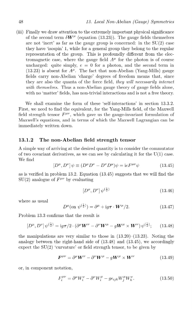
13.1.2 The non-Abelian field strength tensor
A simple way of arriving at the desired quantity is to consider the commutator
of two covariant derivatives, as we can see by calculating it for the U(1) case.
We find
[D
μ , D
ν ] ψ ≡ (D
μ D
ν
− D
ν D
μ )ψ = ieF
μν ψ
(13.45)
as is verified in problem 13.2. Equation (13.45) suggests that we will find the
SU(2) analogue of F
μν by evaluating
1
2
[D
μ , D
ν ] ψ
( )
(13.46)
where as usual
1
2
D
μ (on ψ
( ) ) = ∂
μ + igτ · W
μ /2.
(13.47)
Problem 13.3 confirms that the result is
1
2
1
2
) = igτ /2 · (∂
μ
W
ν
− ∂
ν
W
μ
− gW
μ
× W
ν
[D
μ , D
ν ] ψ
(
) ψ
( ) ;
(13.48)
the manipulations are very similar to those in (13.20)–(13.23). Noting the
analogy between the right-hand side of (13.48) and (13.45), we accordingly
expect the SU(2) ‘curvature’ or field strength tensor, to be given by
F
μν = ∂
μ
W
ν
− ∂
ν
W
μ
− gW
μ
× W
ν
(13.49)
or, in component notation,
μν
μ
μ
F = ∂
μ W
ν
− ∂
ν W
W
ν
(13.50)
i
i
i − g∈ ijk W j k .
13. Local Non-Abelian (Gauge) Symmetries
(iii) Finally we draw attention to the extremely important physical significance
of the second term δW
μ (equation (13.23)). The gauge fields themselves
are not ‘inert’ as far as the gauge group is concerned: in the SU(2) case
they have ‘isospin’ 1, while for a general group they belong to the regular
representation of the group. This is profoundly different from the electromagnetic case, where the gauge field A
μ for the photon is of course
uncharged: quite simply, e = 0 for a photon, and the second term in
(13.23) is absent for A
μ . The fact that non-Abelian (Yang-Mills) gauge
fields carry non-Abelian ‘charge’ degrees of freedom means that, since
they are also the quanta of the force field, they will necessarily interact
with themselves. Thus a non-Abelian gauge theory of gauge fields alone,
with no ‘matter’ fields, has non-trivial interactions and is not a free theory.
We shall examine the form of these ‘self-interactions’ in section 13.3.2.
First, we need to find the equivalent, for the Yang-Mills field, of the Maxwell
field strength tensor F
μν , which gave us the gauge-invariant formulation of
Maxwell’s equations, and in terms of which the Maxwell Lagrangian can be
immediately written down.
13.1.2 The non-Abelian field strength tensor
A simple way of arriving at the desired quantity is to consider the commutator
of two covariant derivatives, as we can see by calculating it for the U(1) case.
We find
[D
μ , D
ν ] ψ ≡ (D
μ D
ν
− D
ν D
μ )ψ = ieF
μν ψ
(13.45)
as is verified in problem 13.2. Equation (13.45) suggests that we will find the
SU(2) analogue of F
μν by evaluating
1
2
[D
μ , D
ν ] ψ
( )
(13.46)
where as usual
1
2
D
μ (on ψ
( ) ) = ∂
μ + igτ · W
μ /2.
(13.47)
Problem 13.3 confirms that the result is
1
2
1
2
) = igτ /2 · (∂
μ
W
ν
− ∂
ν
W
μ
− gW
μ
× W
ν
[D
μ , D
ν ] ψ
(
) ψ
( ) ;
(13.48)
the manipulations are very similar to those in (13.20)–(13.23). Noting the
analogy between the right-hand side of (13.48) and (13.45), we accordingly
expect the SU(2) ‘curvature’ or field strength tensor, to be given by
F
μν = ∂
μ
W
ν
− ∂
ν
W
μ
− gW
μ
× W
ν
(13.49)
or, in component notation,
μν
μ
μ
F = ∂
μ W
ν
− ∂
ν W
W
ν
(13.50)
i
i
i − g∈ ijk W j k .