

46
13. Local Non-Abelian (Gauge) Symmetries
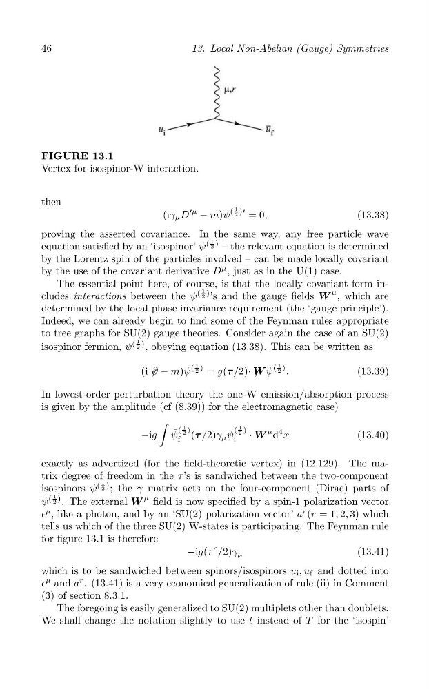
FIGURE 13.1
Vertex for isospinor-W interaction.
then
(iγ μ D
′μ
− m)ψ
(
1 )
2 ′ = 0,
(13.38)
proving the asserted covariance. In the same way, any free particle wave
equation satisfied by an ‘isospinor’ ψ
(
1 )
2
– the relevant equation is determined
by the Lorentz spin of the particles involved – can be made locally covariant
by the use of the covariant derivative D
μ , just as in the U(1) case.
The essential point here, of course, is that the locally covariant form in1
cludes interactions between the ψ
( ) ’s and the gauge fields W
μ
2
, which are
determined by the local phase invariance requirement (the ‘gauge principle’).
Indeed, we can already begin to find some of the Feynman rules appropriate
to tree graphs for SU(2) gauge theories. Consider again the case of an SU(2)
isospinor fermion, ψ
(
1 )
2 , obeying equation (13.38). This can be written as
(i ∂ − m)ψ
(
1 )
2
= g(τ /2)· W ψ
(
1 )
2 .
(13.39)
In lowest-order perturbation theory the one-W emission/absorption process
is given by the amplitude (cf (8.39)) for the electromagnetic case)
∫
−
¯ (
1 )
(
1 )
ig ψ
2
f (τ /2)γ μ ψ
2
i
· W
μ d
4 x
(13.40)
exactly as advertized (for the field-theoretic vertex) in (12.129). The matrix degree of freedom in the τ ’s is sandwiched between the two-component
isospinors ψ
(
1 )
2 ; the γ matrix acts on the four-component (Dirac) parts of
ψ
(
1 )
2 . The external W
μ field is now specified by a spin-1 polarization vector
∈
μ , like a photon, and by an ‘SU(2) polarization vector’ a
r (r = 1, 2, 3) which
tells us which of the three SU(2) W-states is participating. The Feynman rule
for figure 13.1 is therefore
−ig(τ
r /2)γ μ
(13.41)
which is to be sandwiched between spinors/isospinors u i , u ¯ f and dotted into
∈
μ and a
r . (13.41) is a very economical generalization of rule (ii) in Comment
(3) of section 8.3.1.
The foregoing is easily generalized to SU(2) multiplets other than doublets.
We shall change the notation slightly to use t instead of T for the ‘isospin’
/
/
13. Local Non-Abelian (Gauge) Symmetries
FIGURE 13.1
Vertex for isospinor-W interaction.
then
(iγ μ D
′μ
− m)ψ
(
1 )
2 ′ = 0,
(13.38)
proving the asserted covariance. In the same way, any free particle wave
equation satisfied by an ‘isospinor’ ψ
(
1 )
2
– the relevant equation is determined
by the Lorentz spin of the particles involved – can be made locally covariant
by the use of the covariant derivative D
μ , just as in the U(1) case.
The essential point here, of course, is that the locally covariant form in1
cludes interactions between the ψ
( ) ’s and the gauge fields W
μ
2
, which are
determined by the local phase invariance requirement (the ‘gauge principle’).
Indeed, we can already begin to find some of the Feynman rules appropriate
to tree graphs for SU(2) gauge theories. Consider again the case of an SU(2)
isospinor fermion, ψ
(
1 )
2 , obeying equation (13.38). This can be written as
(i ∂ − m)ψ
(
1 )
2
= g(τ /2)· W ψ
(
1 )
2 .
(13.39)
In lowest-order perturbation theory the one-W emission/absorption process
is given by the amplitude (cf (8.39)) for the electromagnetic case)
∫
−
¯ (
1 )
(
1 )
ig ψ
2
f (τ /2)γ μ ψ
2
i
· W
μ d
4 x
(13.40)
exactly as advertized (for the field-theoretic vertex) in (12.129). The matrix degree of freedom in the τ ’s is sandwiched between the two-component
isospinors ψ
(
1 )
2 ; the γ matrix acts on the four-component (Dirac) parts of
ψ
(
1 )
2 . The external W
μ field is now specified by a spin-1 polarization vector
∈
μ , like a photon, and by an ‘SU(2) polarization vector’ a
r (r = 1, 2, 3) which
tells us which of the three SU(2) W-states is participating. The Feynman rule
for figure 13.1 is therefore
−ig(τ
r /2)γ μ
(13.41)
which is to be sandwiched between spinors/isospinors u i , u ¯ f and dotted into
∈
μ and a
r . (13.41) is a very economical generalization of rule (ii) in Comment
(3) of section 8.3.1.
The foregoing is easily generalized to SU(2) multiplets other than doublets.
We shall change the notation slightly to use t instead of T for the ‘isospin’
/
/