

413
K.1. The spin-averaged squared matrix element
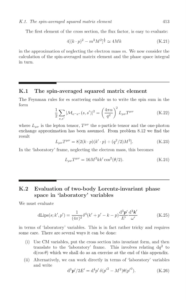
The first element of the cross section, the flux factor, is easy to evaluate:
1
4[(k · p)
2
− m
2 M
2 ] 2 ≃ 4M k
(K.21)
in the approximation of neglecting the electron mass m. We now consider the
calculation of the spin-averaged matrix element and the phase space integral
in turn.
K.1 The spin-averaged squared matrix element
The Feynman rules for es scattering enable us to write the spin sum in the
form
(
) 2
∑
1
4πα
|M e − s + (s, s
′ )|
2 =
L μν T
μν
(K.22)
2 '
q 2
s,s
where L μν is the lepton tensor, T
μν the s-particle tensor and the one-photon
exchange approximation has been assumed. From problem 8.12 we find the
result
L μν T
μν = 8[2(k · p)(k
′
· p) + (q
2 /2)M
2 ].
(K.23)
In the ‘laboratory’ frame, neglecting the electron mass, this becomes
L μν T
μν = 16M
2 kk
′ cos
2 (θ/2).
(K.24)
K.2 Evaluation of two-body Lorentz-invariant phase
space in ‘laboratory’ variables
We must evaluate
′
1
d
3
p d
3
k
′
′
dLips(s; k
′ , p
′ ) ≡
δ
4 (k
′ + p − k − p)
(K.25)
(4π) 2
E ′ ω ′
in terms of ‘laboratory’ variables. This is in fact rather tricky and requires
some care. There are several ways it can be done:
(i) Use CM variables, put the cross section into invariant form, and then
translate to the ‘laboratory’ frame. This involves relating dq to
d(cos θ) which we shall do as an exercise at the end of this appendix.
(ii) Alternatively, we can work directly in terms of ‘laboratory’ variables
and write
′ 2
′ 0
d
3
p
′ /2E
′ = d
4 p
′ δ(p − M
2 )θ(p ).
(K.26)
2
K.1. The spin-averaged squared matrix element
The first element of the cross section, the flux factor, is easy to evaluate:
1
4[(k · p)
2
− m
2 M
2 ] 2 ≃ 4M k
(K.21)
in the approximation of neglecting the electron mass m. We now consider the
calculation of the spin-averaged matrix element and the phase space integral
in turn.
K.1 The spin-averaged squared matrix element
The Feynman rules for es scattering enable us to write the spin sum in the
form
(
) 2
∑
1
4πα
|M e − s + (s, s
′ )|
2 =
L μν T
μν
(K.22)
2 '
q 2
s,s
where L μν is the lepton tensor, T
μν the s-particle tensor and the one-photon
exchange approximation has been assumed. From problem 8.12 we find the
result
L μν T
μν = 8[2(k · p)(k
′
· p) + (q
2 /2)M
2 ].
(K.23)
In the ‘laboratory’ frame, neglecting the electron mass, this becomes
L μν T
μν = 16M
2 kk
′ cos
2 (θ/2).
(K.24)
K.2 Evaluation of two-body Lorentz-invariant phase
space in ‘laboratory’ variables
We must evaluate
′
1
d
3
p d
3
k
′
′
dLips(s; k
′ , p
′ ) ≡
δ
4 (k
′ + p − k − p)
(K.25)
(4π) 2
E ′ ω ′
in terms of ‘laboratory’ variables. This is in fact rather tricky and requires
some care. There are several ways it can be done:
(i) Use CM variables, put the cross section into invariant form, and then
translate to the ‘laboratory’ frame. This involves relating dq to
d(cos θ) which we shall do as an exercise at the end of this appendix.
(ii) Alternatively, we can work directly in terms of ‘laboratory’ variables
and write
′ 2
′ 0
d
3
p
′ /2E
′ = d
4 p
′ δ(p − M
2 )θ(p ).
(K.26)
2